3.7: Change of Variables in Definite Integrals

One of the basic techniques for evaluating an integral in one-variable calculus is substitution, replacing one variable with another in such a way that the resulting integral is of a simpler form. Although slightly more subtle in the case of two or more variables, a similar idea provides a powerful technique for evaluating definite integrals.

Linear change of variables

We will present the main idea through an example. Let

\[ D=\left\{(x, y): 9 x^{2}+4 y^{2} \leq 36\right\} , \nonumber \]

the region inside the ellipse which intersects the \(x\)-axis at (−2,0) and (2,0) and the \(y\)-axis at (0,−3) and (0,3). To find the area of \(D\), we evaluate

\[ \iint_{D} d x d y=\int_{-2}^{2} \int_{-\frac{3}{2} \sqrt{4-x^{2}}}^{\frac{3}{2} \sqrt{4-x^{2}}} d y d x=\int_{-2}^{2} 3 \sqrt{4-x^{2}} d x=6 \pi , \nonumber \]

where the final integral may be evaluated using the substitution \(x=2 \sin (\theta)\) or by noting that

\[ \int_{-2}^{2} \sqrt{4-x^{2}} d x \nonumber \]

is one-half of the area of a circle of radius 2. Alternatively, suppose we write the equation of the ellipse as

\[ \frac{x^{2}}{4}+\frac{y^{2}}{9}=1 \nonumber \]

and make the substitution \(x=2u\) and \(y=3v\). Then \(u = \frac{x}{2} \) and \(v = \frac{y}{3} \), so if \((x,y)\) is a point in \(D\), then

\[ u^{2}+v^{2}=\frac{x^{2}}{4}+\frac{y^{2}}{9} \leq 1 . \nonumber \]

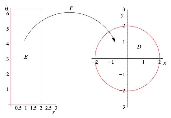
That is, if \((x,y)\) is a point in \(D\), then \((u,v)\) is a point in the unit disk

\[ E=\left\{(u, v): u^{2}+v^{2} \leq 1\right\} . \nonumber \]

Conversely, if \((u,v)\) is a point in \(E\), then

\[ \frac{x^{2}}{4}+\frac{y^{2}}{9}=\frac{4 u^{2}}{4}+\frac{9 v^{2}}{9}=u^{2}+v^{2} \leq 1 , \nonumber \]

so \((x,y)\) is a point in \(D\). Thus the function \(F(u, v)=(2 u, 3 v)\) takes the region \(E\), a closed disk of radius 1, and stretches it onto the region \(D\) (as shown in Figure 3.7.1).

Figure \(\PageIndex{1}\): \(F\) maps \(E\) onto \(D\)

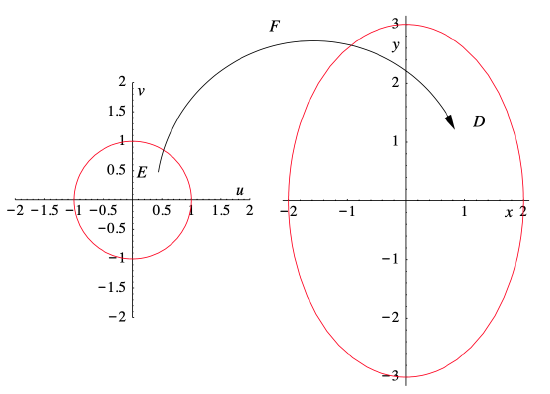
However, note that even though every point in \(E\) corresponds to exactly one point in \(D\), and, conversely, every point in \(D\) corresponds to exactly on point in \(E\), nevertheless \(E\) and \(D\) do not have the same area. To see how \(F\) changes area, consider what it does to the unit square \(S\) with sides \(\mathbf{e}_{1}=(1,0)\) and \(\mathbf{e}_{2}=(0,1)\). The area of \(S\) is 1, but \(F\) maps \(S\) onto a rectangle \(R\) with sides

\[ F(1,0)=(2,0) \nonumber \]

and

\[ F(0,1)=(0,3) \nonumber \]

and area 6. This a special case of a general fact we saw in Section 1.6: the linear function \(F\), with associated matrix

\[ M=\left[\begin{array}{ll}
2 & 0 \\
0 & 3
\end{array}\right] , \nonumber \]

maps the unit square \(S\) onto a parallelogram \(R\) with area

\[ |\operatorname{det}(M)|=6 . \nonumber \]

The important fact for us here is that 1 unit of area in the \(uv\)-plane corresponds to 6 units of area in the \(xy\)-plane. Hence the area of \(D\) will be 6 times the area of \(E\). That is,

\[ \iint_{D} d x d y=\iint_{E}|\operatorname{det}(M)| d u d v=\iint_{E} 6 d u d v=6 \iint_{E} d u d v=6 \pi , \nonumber \]

where the final integral is simply the area inside a circle of radius 1.

These ideas provide the background for a proof of the following theorem.

Theorem \(\PageIndex{1}\)

Suppose \(f: \mathbb{R}^{n} \rightarrow \mathbb{R}\) is continuous on a an open set \(U\) containing the closed bounded set \(D\). Suppose \(F: \mathbb{R}^{n} \rightarrow \mathbb{R}^{n}\) is a linear function, \(M\) is an \(n \times n\) matrix such that \(F(\mathbf{u})=M \mathbf{u}\), and \(\operatorname{det}(M) \neq 0\). If \(F\) maps the region \(E\) onto the region \(D\) and we define the change of variables

\[ \left[\begin{array}{c}
x_{1} \\
x_{2} \\
\vdots \\
x_{n}
\end{array}\right]=M\left[\begin{array}{c}
u_{1} \\
u_{2} \\
\vdots \\
u_{n}
\end{array}\right] , \nonumber \]

then

\[ \begin{align}
\iint \cdots \int_{D} f\left(x_{1}, x_{2}, \ldots, x_{n}\right) d x_{1} d x_{2} \cdots d x_{n} \nonumber \\
&=\iint \cdots \int_{E} f\left(F\left(u_{1}, u_{2}, \ldots, u_{n}\right)\right)|\operatorname{det}(M)| d u_{1} d u_{2} \cdots d u_{n} \label{3.7.1}
\end{align} . \]

Example \(\PageIndex{1}\)

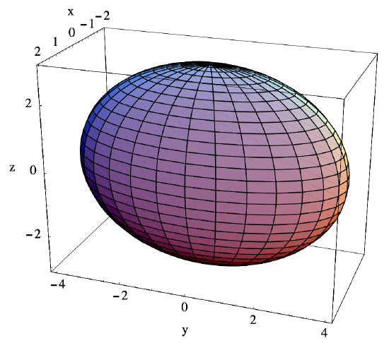
Let \(D\) be the region in \(\mathbb{R}^3\) bounded by the ellipsoid with equation

\[ \frac{x^{2}}{4}+\frac{y^{2}}{16}+\frac{z^{2}}{9}=1 . \nonumber \]

See Figure 3.7.2.

Figure \(\PageIndex{2}\): The ellipsoid \(\frac{x^{2}}{4}+\frac{y^{2}}{16}+\frac{z^{2}}{9}=1\)

If we make the change of variables \(x = 2u, y = 4v\), and \(z = 3w\), that is,

\[ \left[\begin{array}{l}
x \\
y \\
z
\end{array}\right]=\left[\begin{array}{lll}
2 & 0 & 0 \\
0 & 4 & 0 \\
0 & 0 & 3
\end{array}\right]\left[\begin{array}{c}
u \\
v \\
w
\end{array}\right] , \nonumber \]

then, for any \((x,y,z)\) in \(D\), we have

\[ u^{2}+v^{2}+w^{2}=\frac{x^{2}}{4}+\frac{y^{2}}{16}+\frac{z^{2}}{9} \leq 1 . \nonumber \]

That is, if \((x,y,z)\) lies in \(D\), then the corresponding \((u,v,w)\) lies in the closed unit ball \(E=\bar{B}^{3}((0,0,0), 1)\). Conversely, if \((u,v,w)\) lies in \(E\), then

\[ \frac{x^{2}}{4}+\frac{y^{2}}{16}+\frac{z^{2}}{9}=\frac{4 u^{2}}{4}+\frac{16 v^{2}}{16}+\frac{9 w^{2}}{9}=u^{2}+v^{2}+w^{2} \leq 1 , \nonumber \]

so \((x,y,z)\) lies in \(D\). Hence, the change of variables \(F(u, v, w)=(2 u, 4 v, 3 w)\) maps \(E\) onto \(D\). Now

\[ \operatorname{det}\left[\begin{array}{lll}
2 & 0 & 0 \\
0 & 4 & 0 \\
0 & 0 & 3
\end{array}\right]=24 , \nonumber \]

so if \(V\) is the volume of \(D\), then

\[ V=\iiint_{D} d x d y d z=\iiint_{E} 24 d u d v d w=24 \iiint_{E} d u d v d w=24\left(\frac{4 \pi}{3}\right)=32 \pi , \nonumber \]

where we have used the fact that the volume of a sphere of radius 1 is \( \frac{4 \pi }{3} \) to evaluate the final integral.

Nonlinear change of variables

Without going into the technical details, we will indicate how to proceed when the change of variables is not linear. Suppose \(f: \mathbb{R}^{n} \rightarrow \mathbb{R}\) is continuous on a an open set \(U\) containing the closed bounded set \(D\) and \(F: \mathbb{R}^{n} \rightarrow \mathbb{R}^{n}\) maps a closed bounded region \(E\) of \(\mathbb{R}^n\) onto \(D\) so that every point of \(D\) corresponds to exactly one point of \(E\). Writing \(F(\mathbf{u})=\left(F_{1}(\mathbf{u}), F_{2}(\mathbf{u}), \ldots, F_{n}(\mathbf{u})\right) \), we will assume that \(F_{1}, F_{2}, \ldots,\) and \(F_n\) are all differentiable on an open set \(W\) containing \(E\). Although we will not study this type of function until Chapter 4, the natural candidate for the derivative of \(F\) is the matrix whose \(i\)th row is \(\nabla F_{i}(\mathbf{u})\). Letting \(x_{i}=F_{i}\left(u_{1}, u_{2}, \ldots, u_{n}\right)\), \(i=1,2, \ldots, n\), we denote this matrix, called the Jacobian matrix of \(F\),

\[ \frac{\partial\left(x_{1}, x_{2}, \ldots, x_{n}\right)}{\partial\left(u_{1}, u_{2}, \ldots, u_{n}\right)} . \]

Explicitly,

\[ \frac{\partial\left(x_{1}, x_{2}, \ldots, x_{n}\right)}{\partial\left(u_{1}, u_{2}, \ldots, u_{n}\right)}=\left[\begin{array}{cccc}
\frac{\partial}{\partial u_{1}} F_{1}(\mathbf{u}) & \frac{\partial}{\partial u_{2}} F_{1}(\mathbf{u}) & \cdots & \frac{\partial}{\partial u_{n}} F_{1}(\mathbf{u}) \\
\frac{\partial}{\partial u_{1}} F_{2}(\mathbf{u}) & \frac{\partial}{\partial u_{2}} F_{2}(\mathbf{u}) & \cdots & \frac{\partial}{\partial u_{n}} F_{2}(\mathbf{u}) \\
\vdots & \vdots & \ddots & \vdots \\
\frac{\partial}{\partial u_{1}} F_{n}(\mathbf{u}) & \frac{\partial}{\partial u_{2}} F_{n}(\mathbf{u}) & \cdots & \frac{\partial}{\partial u_{n}} F_{n}(\mathbf{u})
\end{array}\right] . \]

We shall see in Chapter 4 that

\[ \frac{\partial\left(x_{1}, x_{2}, \ldots, x_{n}\right)}{\partial\left(u_{1}, u_{2}, \ldots, u_{n}\right)} \nonumber \]

is the matrix for the linear part of the best affine approximation to \(F\) at \(\left(u_{1}, u_{2}, \ldots, u_{n}\right)\). Hence, for sufficiently small rectangles, the factor by which \(F\) changes the area of a rectangle when it maps it to a region will be approximately

\[ \left|\operatorname{det} \frac{\partial\left(x_{1}, x_{2}, \ldots, x_{n}\right)}{\partial\left(u_{1}, u_{2}, \ldots, u_{n}\right)}\right| . \]

One may then show that, analogous to (\(\ref{3.7.1}\)), we have

\[ \begin{align}
\int \cdots & \iint_{D} f\left(x_{1}, x_{2}, \ldots, x_{n}\right) d x_{1} d x_{2} \cdots d x_{n} \nonumber \\
&=\int \cdots \iint_{E} f\left(F\left(u_{1}, u_{2}, \ldots, u_{n}\right)\right)\left|\operatorname{det} \frac{\partial\left(x_{1}, x_{2}, \ldots, x_{n}\right)}{\partial\left(u_{1}, u_{2}, \ldots, u_{n}\right)}\right| d u_{1} d u_{2} \cdots d u_{n}. \label{3.7.5}
\end{align} \]

Note that (\(\ref{3.7.5}\)) is just (\(\ref{3.7.1}\)) with the matrix \(M\) replaced by the Jacobian of \(F\).

We will now look at two very useful special cases of the preceding result. See Exercises 22 and 23 for a third special case.

Polar coordinates

As an alternative to describing the location of a point \(P\) in the plane using its Cartesian coordinates \((x,y)\), we may locate the point using \(r\), the distance from \(P\) to the origin, and \(\theta\), the angle between the vector from (0,0) to \(P\) and the positive \(x\)-axis, measured in the counterclockwise direction from 0 to \(2 \pi \) (see Figure 3.7.3).

Figure \(\PageIndex{3}\): Polar and Cartesian coordinates for a point \(P\)

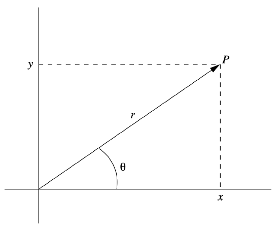
That is, if \(P\) has Cartesian coordinates \((x,y)\), with \(x \neq 0\), we may define its polar coordinates \((r, \theta )\) by specifying that

\[ r=\sqrt{x^{2}+y^{2}} \]

and

\[ \tan (\theta)=\frac{y}{x} , \]

where we take \(0 \leq \theta \leq \pi\) if \(y \geq 0\) and \(\pi<\theta<2 \pi\) if \(y<0\). If \(x=0\), we let \(\theta = \frac{\pi}{2}\) if \(y>0\) and \( \theta = \frac{3 \pi}{2}\) if \(y<0\). For \((x, y)=(0,0), r=0\) and \(\theta\) could have any value, and so is undefined. Conversely, if a point \(P\) has polar coordinates \((r, \theta )\), then

\[ x=r \cos (\theta) \]

and

\[ y=r \sin (\theta) . \]

Note that the choice of the interval \( [0,2 \pi) \) for the values of \(\theta\) is not unique, with any interval of length \(2 \pi \) working as well. Although \( [0,2 \pi) \) is the most common choice for values of \(\theta \), it is sometimes useful to use \(( - \pi , \pi ) \) instead.

Example \(\PageIndex{2}\)

If a point \(P\) has Cartesian coordinates (−1,1), then its polar coordinates are \(\left(\sqrt{2}, \frac{3 \pi}{4}\right)\).

Example \(\PageIndex{3}\)

A point with polar coordinates \(\left(3, \frac{\pi}{6}\right)\) has Cartesian coordinates \(\left(\frac{3 \sqrt{3}}{2}, \frac{3}{2}\right)\).

In our current context, we want to think of the polar coordinate mapping

\[(x, y)=F(r, \theta)=(r \cos (\theta), r \sin (\theta)) \]

as a change of variables between the \(r \theta \)-plane and the \(xy\)-plane. This mapping is particularly useful for us because it maps rectangular regions in the \(r \theta \)-plane onto circular regions in the \(xy\)-plane. For example, for any \(a>0\), \(F\) maps the rectangular region

\[ E=\{(r, \theta): 0 \leq r \leq a, 0 \leq \theta<2 \pi\} \nonumber \]

in the \(r \theta \)-plane onto the closed disk

\[ D=\bar{B}^{2}((0,0), a)=\left\{(x, y): x^{2}+y^{2} \leq a\right\} \nonumber \]

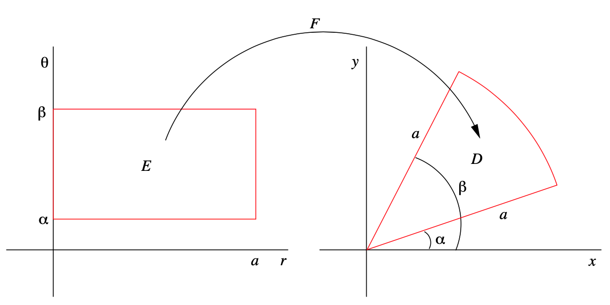
in the \(xy\)-plane (see Figure 3.7.5 below for an example). More generally, for any \( 0 \leq \alpha < \beta < 2 \pi \), \(F\) maps the rectangular region

\[ E=\{(r, \theta): 0 \leq r \leq a, \alpha \leq \theta<\beta\} \nonumber \]

in the \(r \theta \)-plane onto a region \(D\) in the \(xy\)-plane which is the sector of the closed disk \(\bar{B}^{2}((0,0), a)\) which lies between radii of angles \(\alpha \) and \(\beta \) (see Figure 3.7.4).

Figure \(\PageIndex{4}\): Polar coordinate change of variables

Figure \(\PageIndex{5}\): Polar coordinate change of variables maps \([0,2] \times[0,2 \pi]\) to \(\bar{B}^{2}((0,0), 2)\)

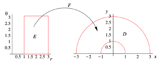
Another basic example is an annulus: for any \(0 < a < b\), \(F\) maps the rectangular region

\[ E=\{(r, \theta): a \leq r \leq b, 0 \leq \theta<2 \pi\} \nonumber \]

in the \(r \theta \)-plane onto the annulus

\[ D=\left\{(x, y): a \leq x^{2}+y^{2} \leq b\right\} \nonumber \]

in the \(xy\)-plane. Figure 3.7.6 illustrates this mapping for the upper half of an annulus.

Figure \(\PageIndex{6}\): Polar coordinates map \([1,3] \times[0, \pi]\) to top half of an annulus

Example \(\PageIndex{4}\)

Let \(V\) be the volume of the region which lies beneath the paraboloid with equation \(z=4-x^{2}-y^{2}\) and above the \(xy\)-plane. In Section 3.6, we saw that

\[ V=\iint_{D}\left(4-x^{2}-y^{2}\right) d x d y=8 \pi , \nonumber \]

where

\[ D=\left\{(x, y): x^{2}+y^{2} \leq 4\right\} . \nonumber \]

The use of polar coordinates greatly simplifies the evaluation of this integral. With the polar coordinate change of variables

\[ x=r \cos (\theta) \nonumber \]

and

\[ y=r \sin (\theta) , \nonumber \]

the closed disk \(D\) in the \(xy\)-plane corresponds to the closed rectangle

\[ E=\{(r, \theta): 0 \leq r \leq 2,0 \leq \theta \leq 2 \pi\} \nonumber \]

in the \(r \theta \)-plane (see Figure 3.7.5 above). Note that in describing \(E\) we have allowed \(\theta = 2 \pi \), but this has no affect on our outcome since a line has no area in \(\mathbb{R}^2\). Moreover, if we let \(f(x, y)=4-x^{2}-y^{2}\), then

\[ \begin{aligned}
f(F(r, \theta)) &=f(r \cos (\theta), r \sin (\theta)) \\
&=4-r^{2} \cos ^{2}(\theta)-r^{2} \sin (\theta) \\
&=4-r^{2}\left(\cos ^{2}(\theta)+\sin ^{2}(\theta)\right.\\
&=4-r^{2},
\end{aligned} \]

which also follows from the fact that \(r^{2}=x^{2}+y^{2}\). Now

\[ \frac{\partial(x, y)}{\partial(r, \theta)}=\left[\begin{array}{ll}
\frac{\partial}{\partial r} r \cos (\theta) & \frac{\partial}{\partial \theta} r \cos (\theta) \\
\frac{\partial}{\partial r} r \sin (\theta) & \frac{\partial}{\partial \theta} r \sin (\theta)
\end{array}\right]=\left[\begin{array}{cr}
\cos (\theta) & -r \sin (\theta) \\
\sin (\theta) & r \cos (\theta)
\end{array}\right] , \]

so

\[ \operatorname{det} \frac{\partial(x, y)}{\partial(r, \theta)}=r \cos ^{2}(\theta)+r \sin ^{2}(\theta)=r\left(\cos ^{2}(\theta)+\sin ^{2}(\theta)\right)=r . \]

Hence, using (\(\ref{3.7.5}\)), we have

\[ \begin{aligned}
\iint_{D}\left(4-x^{2}-y^{2}\right) d x d y &=\iint_{E}\left(4-r^{2}\right)\left|\operatorname{det} \frac{\partial(x, y)}{\partial(r, \theta)}\right| d r d \theta \\
&=\int_{0}^{2} \int_{0}^{2 \pi}\left(4-r^{2}\right) r d \theta d r \\
&=\int_{0}^{2} 2 \pi\left(4 r-r^{3}\right) d r \\
&=\left.2 \pi\left(2 r^{2}-\frac{r^{4}}{4}\right)\right|_{0} ^{2} \\
&=2 \pi(8-4) \\
&=8 \pi .
\end{aligned} \]

Example \(\PageIndex{5}\)

Suppose \(D\) is the part of the region between the circles with equations \(x^2 + y^2 = 1\) and \(x^2 + y^2 = 9\) which lies above the \(x\)-axis. That is,

\[ D=\left\{(x, y): 1 \leq x^{2}+y^{2} \leq 9, x \geq 0\right\} . \nonumber \]

We wish to evaluate

\[ \iint_{D} e^{-\left(x^{2}+y^{2}\right)} d x d y . \nonumber \]

Under the polar coordinate change of variables

\[ x=r \cos (\theta) \nonumber \]

and

\[ y=r \sin (\theta) , \nonumber \]

the annular region \(D\) corresponds to the closed rectangle

\[ E=\{(r, \theta): 1 \leq r \leq 3,0 \leq \theta \leq \pi\} , \nonumber \]

as illustrated in Figure 3.7.6 above. Moreover, \(x^2 + y^2 = r^2\) and, as we saw in the previous example,

\[ \left|\operatorname{det} \frac{\partial(x, y)}{\partial(r, \theta)}\right|=r . \nonumber \]

Hence

\[ \begin{aligned}
\iint_{D} e^{-\left(x^{2}+y^{2}\right)} d x d y &=\iint_{E} r e^{-r^{2}} d r d \theta \\
&=\int_{1}^{3} \int_{0}^{\pi} r e^{-r^{2}} d \theta d r \\
&=\int_{1}^{3} \pi r e^{-r^{2}} d r \\
&=-\left.\frac{\pi}{2} e^{-r^{2}}\right|_{1} ^{3} \\
&=\frac{\pi}{2}\left(e^{-1}-e^{-9}\right) .
\end{aligned} \]

Note that in this case the change of variables not only simplified the region of integration, but also put the function being integrated into a form to which we could apply the Fundamental Theorem of Calculus.

Spherical coordinates

Next consider the following extension of polar coordinates to three space: given a point \(P\) with Cartesian coordinates \((x,y,z)\), let \(\rho\) be the distance from \(P\) to the origin, \( \theta \) be the angle coordinate for the polar coordinates of \((x,y,0)\) (the projection of \(P\) onto the \(xy\)-plane), and let \(\varphi \) be the angle between the vector from the origin to \(P\) and the positive \(z\)-axis, measured from 0 to \(\pi \). If \(x \neq 0 \), we have

\[ \rho=\sqrt{x^{2}+y^{2}+z^{2}} , \]

\[ \tan (\theta)=\frac{y}{x} , \]

and

\[ \cos (\varphi)=\frac{z}{\sqrt{x^{2}+y^{2}+z^{2}}} , \]

where \(0 \leq \theta<2 \pi\) and \(0 \leq \varphi \leq \pi\). As with polar coordinates, if \(x=0\) we let \(\theta = \frac{\pi}{2}\) if \(y>0\), \(\theta = \frac{3 \pi}{2}\) if \(y<0\), and \(\theta\) is undefined if \(y=0\). See Figure 3.7.7.

Figure \(\PageIndex{7}\): Spherical and Cartesian coordinates for a point \(P\)

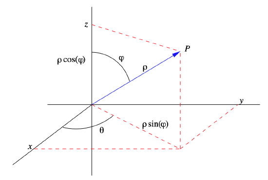
Conversely, given a point \(P\) with spherical coordinates \(( \rho , \theta , \varphi )\), the projection of \(P\) onto the \(xy\)-plane will have polar coordinate \(r=\rho \sin (\varphi)\). Hence the Cartesian coordinates of \(P\) are

\[ x=\rho \cos (\theta) \sin (\varphi) , \]

\[ y=\rho \sin (\theta) \sin (\varphi) , \]

and

\[ z=\rho \cos (\varphi) . \]

Example \(\PageIndex{6}\)

If a point \(P\) has Cartesian coordinates (2,−2,1), then its spherical coordinates satisfy

\[ \rho=\sqrt{4+4+1}=3 , \nonumber \]

\[ \tan (\theta)=\frac{-2}{2}=-1 , \nonumber \]

and

\[ \cos (\varphi)=\frac{1}{\sqrt{4+4+1}}=\frac{1}{3} . \nonumber \]

Hence we have

\[ \theta=\frac{7 \pi}{4} \nonumber \]

and

\[ \varphi=\cos ^{-1}\left(\frac{1}{3}\right)=1.2310 , \nonumber \]

where we have rounded the value of \(\varphi \) to four decimal places. Hence \(P\) has spherical coordinates \(\left(3, \frac{7 \pi}{4}, 1.2310\right)\).

Example \(\PageIndex{7}\)

If a point \(P\) has spherical coordinates \(\left(4, \frac{\pi}{3}, \frac{3 \pi}{4}\right)\), then its Cartesian coordinates are

\[ x=4 \cos \left(\frac{\pi}{3}\right) \sin \left(\frac{3 \pi}{4}\right)=4\left(\frac{1}{2}\right)\left(\frac{1}{\sqrt{2}}\right)=\sqrt{2} , \nonumber \]

\[ y=4 \sin \left(\frac{\pi}{3}\right) \sin \left(\frac{3 \pi}{4}\right)=4\left(\frac{\sqrt{3}}{2}\right)\left(\frac{1}{\sqrt{2}}\right)=\sqrt{6} , \nonumber \]

and

\[ z=4 \cos \left(\frac{3 \pi}{4}\right)=4\left(-\frac{1}{\sqrt{2}}\right)=-2 \sqrt{2} . \nonumber \]

Analogous to our work with polar coordinates, we think of the spherical coordinate mapping

\[ (x, y, z)=F(\rho, \theta, \varphi)=(\rho \cos (\theta) \sin (\varphi), \rho \sin (\theta) \sin (\varphi), \rho \cos (\varphi)) \label{3.7.19} \]

as a change of variables between \(\rho \theta \varphi \)-space and \(xyz\)-space. This mapping is particularly useful for evaluating triple integrals because it maps rectangular regions in \(\rho \theta \varphi \)-space onto spherical regions in \(xyz\)-space. For the most basic example, for any \(a>0\), \(F\) maps the rectangular region

\[ E=\{(\rho, \theta, \varphi): 0 \leq \rho \leq a, 0 \leq \theta<2 \pi, 0 \leq \varphi \leq \pi\} \nonumber \]

in \(\rho \theta \varphi \)-space onto the closed ball

\[ D=\bar{B}^{3}((0,0,0), a)=\left\{(x, y, z): x^{2}+y^{2}+z^{2} \leq a\right\} \nonumber \]

in \(xyz\)-space. More generally, for any \(0<a<b, 0 \leq \alpha<\beta<2 \pi\), and \(0 \leq \gamma<\delta \leq \pi, F\) maps the rectangular region

\[ E=\{(\rho, \theta, \varphi): a \leq \rho \leq b, \alpha \leq \theta<\beta, \gamma \leq \varphi \leq \delta\} \nonumber \]

onto a region \(D\) in \(xyz\)-space which lies between the concentric spheres \(S^{2}((0,0,0), a)\) and \(S^{2}((0,0,0), b)\), and for which the angle \(\theta \) lies between \(\alpha\) and \(\beta\) and the angle \(\varphi\) between \(\gamma\) and \(\delta\). For example, if \(\alpha=0, \beta=\pi, \gamma=0\), and \(\delta = \frac{\pi}{2}\), then \(D\) is one-half of the region lying between two concentric hemispheres with radii \(a\) and \(b\).

Before using the spherical coordinate change of variable in (\(\ref{3.7.19}\)) to evaluate an integral using (\(\ref{3.7.5}\)), we need to compute the determinate of the Jacobian of \(F\). Now

\[ \begin{align}
\frac{\partial(x, y, z)}{\partial(\rho, \theta, \varphi)}=&\left[\begin{array}{ccc}
\frac{\partial}{\partial \rho} \rho \cos (\theta) \sin (\varphi) & \frac{\partial}{\partial \theta} \rho \cos (\theta) \sin (\varphi) & \frac{\partial}{\partial \varphi} \rho \cos (\theta) \sin (\varphi) \nonumber \\
\frac{\partial}{\partial \rho} \rho \sin (\theta) \sin (\varphi) & \frac{\partial}{\partial \theta} \rho \sin (\theta) \sin (\varphi) & \frac{\partial}{\partial \varphi} \rho \sin (\theta) \sin (\varphi) \nonumber \\
\frac{\partial}{\partial \rho} \rho \cos (\varphi) & \frac{\partial}{\partial \theta} \rho \cos (\varphi) & \frac{\partial}{\partial \varphi} \rho \cos (\varphi)
\end{array}\right] \nonumber \\
&=\left[\begin{array}{ccc}
\cos (\theta) \sin (\varphi) & -\rho \sin (\theta) \sin (\varphi) & \rho \cos (\theta) \cos (\varphi) \nonumber \\
\sin (\theta) \sin (\varphi) & \rho \cos (\theta) \sin (\varphi) & \rho \sin (\theta) \cos (\varphi) \nonumber \\
\cos (\varphi) & 0 & -\rho \sin (\varphi) \nonumber
\end{array}\right] \label{}
\end{align} \]

so, expanding along the third row,

\[ \begin{align}
\operatorname{det} \frac{\partial(x, y, z)}{\partial(\rho, \theta, \varphi)}=& \cos (\varphi)\left(-\rho^{2} \sin ^{2}(\theta) \sin (\varphi) \cos (\varphi)-\rho^{2} \cos ^{2}(\theta) \sin (\varphi) \cos (\varphi)\right) \nonumber \\
&-\rho \sin (\varphi)\left(\rho \cos ^{2}(\theta) \sin ^{2}(\varphi)+\rho \sin ^{2}(\theta) \sin ^{2}(\varphi)\right. \nonumber \\
=&-\rho^{2} \sin (\varphi) \cos ^{2}(\varphi)\left(\sin ^{2}(\theta)+\cos ^{2}(\theta)\right)-\rho^{2} \sin ^{3}(\varphi)\left(\sin ^{2}(\theta)+\cos ^{2}(\theta)\right) \nonumber \\
=&-\rho^{2} \sin (\varphi) \cos ^{2}(\varphi)-\rho^{2} \sin ^{3}(\varphi) \nonumber \\
=&-\rho^{2} \sin (\varphi)\left(\cos ^{2}(\varphi)+\sin ^{2}(\varphi)\right) \nonumber \\
=&-\rho^{2} \sin (\varphi) \label{}
\end{align} \]

Now \(\rho \geq 0\) and, since \(0 \leq \varphi \leq \pi, \sin (\varphi) \geq 0\), so

\[ \left|\frac{\partial(x, y, z)}{\partial(\rho, \theta, \varphi)}\right|=\rho^{2} \sin (\varphi) . \label{3.7.22} \]

Example \(\PageIndex{8}\)

In an earlier example we used the fact that the volume of a sphere of radius 1 is \(\frac{4 \pi}{3}\). In this example we will verify that the volume of a sphere of radius \(a\) is \(\frac{4}{3} \pi a^{3}\). Let \(V\) be the volume of

\[ D=\bar{B}^{3}((0,0,0), a) , \nonumber \]

the closed ball of radius \(a\) centered at the origin in \(\mathbb{R}^3\). Then

\[ V=\iiint_{D} d x d y d z . \nonumber \]

Although we may evaluate this integral using Cartesian coordinates, we will find it significantly easier to use spherical coordinates. Using the spherical coordinate change of variables

\[ \begin{aligned}
&x=\rho \cos (\theta) \sin (\varphi), \\
&y=\rho \sin (\theta) \sin (\varphi),
\end{aligned} \]

and

\[ z=\rho \cos (\varphi) , \nonumber \]

the region \(D\) in \(xyz\)-space corresponds to the region

\[ E=\{(\rho, \theta, \varphi): 0 \leq \rho \leq a, 0 \leq \theta \leq 2 \pi, 0 \leq \varphi \leq \pi\} \nonumber \]

in \(\rho \theta \varphi \)-space. Using (\(\ref{3.7.22}\)) in the change of variables formula (\(\ref{3.7.5}\)), we have

\[ \begin{aligned}
V &=\iiint_{D} d x d y d z \\
&=\iiint_{E}\left|\operatorname{det} \frac{\partial(x, y, z)}{\partial(\rho, \theta, \varphi)}\right| d \rho d \theta d \varphi \\
&=\int_{0}^{1} \int_{0}^{2 \pi} \int_{0}^{\pi} \rho^{2} \sin (\varphi) d \varphi d \theta d \rho \\
&=\left.\int_{0}^{a} \int_{0}^{2 \pi}\left(-\rho^{2} \cos (\varphi)\right)\right|_{0} ^{\pi} d \theta d \rho \\
&=\int_{0}^{a} \int_{0}^{2 \pi}\left(-\rho^{2}(-1-1)\right) d \theta d \rho \\
&=2 \int_{0}^{a} \int_{0}^{2 \pi} \rho^{2} d \theta d \rho \\
&=4 \pi \int_{0}^{a} \rho^{2} d \rho \\
&=\left.\frac{4 \pi}{3} \rho^{3}\right|_{0} ^{a} \\
&=\frac{4}{3} \pi a^{3} .
\end{aligned} \]

Example \(\PageIndex{9}\)

Suppose we wish to evaluate

\[ \iiint_{D} \log \sqrt{x^{2}+y^{2}+z^{2}} d x d y d z , \nonumber \]

where \(D\) is the region in \(\mathbb{R}^3\) which lies between the two spheres with equations \(x^{2}+y^{2}+z^{2}=1\) and \(x^{2}+y^{2}+z^{2}=4\) and above the \(xy\)-plane. Under the spherical coordinate change of variables

\[ x=\rho \cos (\theta) \sin (\varphi) , \nonumber \]

\[ y=\rho \sin (\theta) \sin (\varphi) , \nonumber \]

and

\[ z=\rho \cos (\varphi) , \nonumber \]

the region \(D\) in \(xyz\)-space corresponds to the region

\[ E=\left\{(\rho, \theta, \varphi): 1 \leq \rho \leq 2,0 \leq \theta \leq 2 \pi, 0 \leq \varphi \leq \frac{\pi}{2}\right\} \nonumber \]

in \(\rho \theta \varphi \)-space. Using (\(\ref{3.7.22}\)) in the change of variables formula (\(\ref{3.7.5}\)), we have

\[ \begin{aligned}
\iiint_{D} \log \sqrt{x^{2}+y^{2}+z^{2}} d x d y d z &=\iiint_{E} \log (\rho)\left|\frac{\partial(x, y, z)}{\partial(\rho, \theta, \varphi)}\right| d \rho d \theta d \varphi \\
&=\int_{1}^{2} \int_{0}^{2 \pi} \int_{0}^{\frac{\pi}{2}} \rho^{2} \log (\rho) \sin (\varphi) d \varphi d \theta d \rho \\
&=\left.\int_{1}^{2} \int_{0}^{2 \pi}\left(-\rho^{2} \log (\rho) \cos (\varphi)\right)\right|_{0} ^{\frac{\pi}{2}} d \theta d \rho \\
&=\int_{1}^{2} \int_{0}^{2 \pi}\left(-\rho^{2} \log (\rho)\right)(0-1) d \theta d \rho \\
&=\int_{1}^{2} \int_{0}^{2 \pi} \rho^{2} \log (\rho) d \theta d \rho \\
&=2 \pi \int_{1}^{2} \rho^{2} \log (\rho) d \rho .
\end{aligned} \]

We use integration by parts to evaluate this final integral: letting

\[ u = log(\rho) \\ dv = \rho^2 d \rho \\ \\ du = \frac{1}{\rho} d \rho \\ v = \frac{\rho^3 }{3}, \nonumber \]

we have

\[ \begin{aligned}
\iiint_{D} \log \sqrt{x^{2}+y^{2}+z^{2}} d x d y d z &=2 \pi\left(\left.\frac{1}{3} \rho^{3} \log (\rho)\right|_{1} ^{2}-\frac{1}{3} \int_{1}^{2} \rho^{2} d \rho\right) \\
&=\frac{16}{3} \pi \log (2)-\left.\frac{2 \pi \rho^{3}}{9}\right|_{1} ^{2} \\
&=\frac{16}{3} \pi \log (2)-\frac{14 \pi}{9} \\
&=\frac{2 \pi}{3}\left(8 \log (2)-\frac{7}{3}\right) .
\end{aligned} \]