7.2: Qualitative Behavior of Solutions to Differential Equations

Last updated
Save as PDF

Page ID: 4335

$ \newcommand{\vecs}[1]{\overset { \scriptstyle \rightharpoonup} {\mathbf{#1}} } $ $ \newcommand{\vecd}[1]{\overset{-\!-\!\rightharpoonup}{\vphantom{a}\smash {#1}}} $$\newcommand{\id}{\mathrm{id}}$ $ \newcommand{\Span}{\mathrm{span}}$ $ \newcommand{\kernel}{\mathrm{null}\,}$ $ \newcommand{\range}{\mathrm{range}\,}$ $ \newcommand{\RealPart}{\mathrm{Re}}$ $ \newcommand{\ImaginaryPart}{\mathrm{Im}}$ $ \newcommand{\Argument}{\mathrm{Arg}}$ $ \newcommand{\norm}[1]{\| #1 \|}$ $ \newcommand{\inner}[2]{\langle #1, #2 \rangle}$ $ \newcommand{\Span}{\mathrm{span}}$ $\newcommand{\id}{\mathrm{id}}$ $ \newcommand{\Span}{\mathrm{span}}$ $ \newcommand{\kernel}{\mathrm{null}\,}$ $ \newcommand{\range}{\mathrm{range}\,}$ $ \newcommand{\RealPart}{\mathrm{Re}}$ $ \newcommand{\ImaginaryPart}{\mathrm{Im}}$ $ \newcommand{\Argument}{\mathrm{Arg}}$ $ \newcommand{\norm}[1]{\| #1 \|}$ $ \newcommand{\inner}[2]{\langle #1, #2 \rangle}$ $ \newcommand{\Span}{\mathrm{span}}$$\newcommand{\AA}{\unicode[.8,0]{x212B}}$

Learning Objectives

In this section, we strive to understand the ideas generated by the following important questions:

What is a slope field?
How can we use a slope field to obtain qualitative information about the solutions of a differential equation?
What are stable and unstable equilibrium solutions of an autonomous differential equation?

In earlier work, we have used the tangent line to the graph of a function $f$ at a point $a$ to approximate the values of $f$ near $a$. The usefulness of this approximation is that we need to know very little about the function; armed with only the value $f (a)$ and the derivative $f' (a)$, we may find the equation of the tangent line and the approximation

\[f (x) \approx f (a) + f 0 (a)(x - a).\]

Remember that a first-order differential equation gives us information about the derivative of an unknown function. Since the derivative at a point tells us the slope of the tangent line at this point, a differential equation gives us crucial information about the tangent lines to the graph of a solution. We will use this information about the tangent lines to create a slope field for the differential equation, which enables us to sketch solutions to initial value problems. Our aim will be to understand the solutions qualitatively. That is, we would like to understand the basic nature of solutions, such as their long-range behavior, without precisely determining the value of a solution at a particular point.

Preview Activity $\PageIndex{1}$

Let’s consider the initial value problem

\[\dfrac{dy}{dt} = t - 2 \nonumber\]

with $y(0) = 1.$

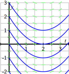
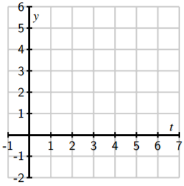
Use the differential equation to find the slope of the tangent line to the solution $y(t)$ at $t = 0$. Then use the initial value to find the equation of the tangent line at $t = 0$. Sketch this tangent line over the interval $-0.25 \leq t \leq 0.25$ on the axes provided.

$alt$

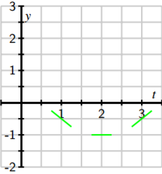
Also shown in the given figure are the tangent lines to the solution $y(t)$ at the points $t = 1$, $2$, and $3$ (we will see how to find these later). Use the graph to measure the slope of each tangent line and verify that each agrees with the value specified by the differential equation.
Using these tangent lines as a guide, sketch a graph of the solution $y(t)$ over the interval $0 ≤ t ≤ 3$ so that the lines are tangent to the graph of $y(t)$.
Use the Fundamental Theorem of Calculus to find $y(t)$, the solution to this initial value problem.
Graph the solution you found in (d) on the axes provided, and compare it to the sketch you made using the tangent lines.

Slope fields

Preview Activity $\PageIndex{1}$ shows that we may sketch the solution to an initial value problem if we know an appropriate collection of tangent lines. Because we may use a given differential equation to determine the slope of the tangent line at any point of interest, by plotting a useful collection of these, we can get an accurate sense of how certain solution curves must behave. Let’s continue looking at the differential equation $\dfrac{dy}{dt} = t - 2. $. If $t = 0$, this equation says that $\dfrac{dy}{dt} = 0 - 2 = -2.$

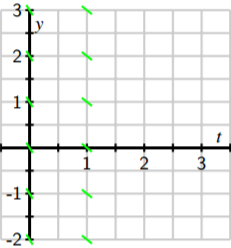
Note that this value holds regardless of the value of $y$. We will therefore sketch tangent lines for several values of $y$ and $t = 0$ with a slope of $-2$.

$alt$

Let’s continue in the same way: if $t = 1$, the Equation tells us that $\dfrac{dy}{dt }= 1 - 2 = -1$ and this holds regardless of the value of $y$. We now sketch tangent lines for several values of $y$ and $t = 1$ with a slope of $-1$.

$alt$

Similarly, we see that when $t = 2$, $dy/dt = 0$ and when $t = 3$, $dy/dt = 1$. We may therefore add to our growing collection of tangent line plots to achieve the next figure.

$alt$

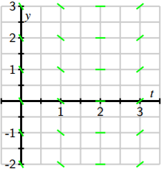
In this figure, you may see the solutions to the differential equation emerge. However, for the sake of clarity, we will add more tangent lines to provide the more complete picture shown below.

$alt$

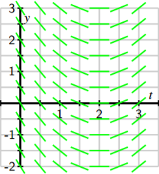
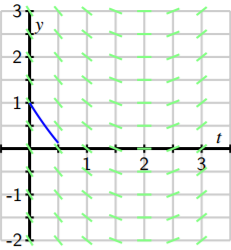
This most recent figure, which is called a slope field for the differential equation, allows us to sketch solutions just as we did in the preview activity. Here, we will begin with the initial value $y(0) = 1$ and start sketching the solution by following the tangent line, as shown in the next figure.

$alt$

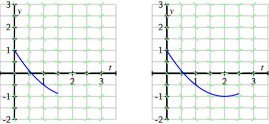
We then continue using this principle: whenever the solution passes through a point at which a tangent line is drawn, that line is tangent to the solution. Doing so leads us to the following sequence of images.

$alt$ $alt$ $alt$

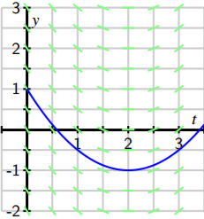
In fact, we may draw solutions for any possible initial value, and doing this for several different initial values for $y(0)$ results in the graphs shown next.

Just as we have done for the most recent example with the equation, we can construct a slope field for any differential equation of interest. The slope field provides us with visual information about how we expect solutions to the differential equation to behave.

Activity $\PageIndex{1}$

Consider the autonomous differential equation

$\dfrac{dy}{dt} = -\dfrac{1}{2} (y - 4).$

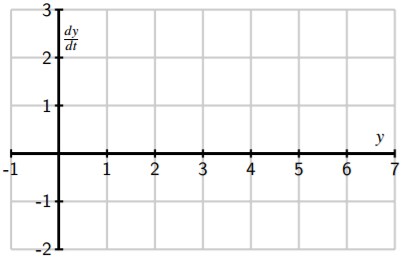
Make a plot of $\dfrac{dy}{dt}$ versus $y$ on the axes provided. Looking at the graph, for what values of $y$ does $y$ increase and for what values of $y$ does $y$ decrease?

$alt$

Next, sketch the slope field for this differential equation on the axes provided.

$alt$

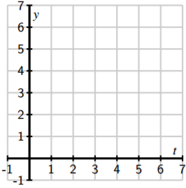
Use your work in (b) to sketch the solutions that satisfy $y(0) = 0$, $y(0) = 2$, $y(0) = 4$, and $y(0) = 6$.
Verify that $y(t) = 4 + 2e^{-t/2}$ is a solution to the given differential equation with the initial value $y(0) = 6$. Compare its graph to the one you sketched in (c).
What is special about the solution where $y(0) = 4$?

Equilibrium Solutions and Stability

As our work in Activity $\PageIndex{1}$ demonstrates, first-order autonomous solutions may have solutions that are constant. In fact, these are quite easy to detect by inspecting the differential equation $dy/dt = f (y)$: constant solutions necessarily have a zero derivative so $dy/dt = 0 = f (y)$. For example, in Activity $\PageIndex{1}$, we considered the equation

\[\dfrac{dy}{dt} = f (y) = - \dfrac{1}{2} (y - 4).\]

Constant solutions are found by setting $f (y) = - \dfrac{1}{2} (y - 4) = 0,$ which we immediately see implies that $y = 4$. Values of $y$ for which $f (y) = 0$ in an autonomous differential equation $\dfrac{dy}{ dt} = f (y) $ are usually called the equilibrium solutions of the differential equation.

Activity $\PageIndex{2}$

Consider the autonomous differential equation

\[\dfrac{dy}{dt} = - \dfrac{1}{2} y(y - 4).\]

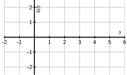
Make a plot of $\frac{dy}{dt}$ versus $y$. Looking at the graph, for what values of $y$ does $y$ increase and for what values of $y$ does $y$ decrease?

$alt$

Identify any equilibrium solutions of the given differential equation.
Now sketch the slope field for the given differential equation.

$alt$

Sketch the solutions to the given differential equation that correspond to initial values $y(0) = -1, 0, 1, \ldots, 5$.
An equilibrium solution $\bar{y}$ is called stable if nearby solutions converge to $\bar{y}$. This means that if the initial condition varies slightly from $y$, then \[\lim_{t→∞} y(t) = \bar{y}.\]Conversely, an equilibrium solution $\bar{y}$ is called unstable if nearby solutions are pushed away from $\bar{y}$. Using your work above, classify the equilibrium solutions you found in (b) as either stable or unstable.
Suppose that $y(t)$ describes the population of a species of living organisms and that the initial value $y(0)$ is positive. What can you say about the eventual fate of this population?
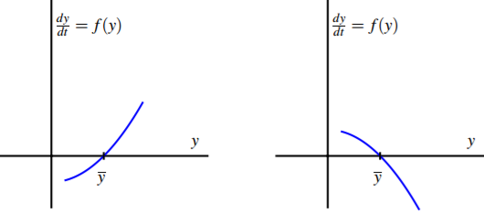
Remember that an equilibrium solution $y$ satisfies f (y) = 0. If we graph $dy/dt = f (y)$ as a function of $y$, for which of the following differential equations is $y$ a stable equilibrium and for which is $y$ unstable? Why?

$alt$

Summary

In this section, we encountered the following important ideas:

A slope field is a plot created by graphing the tangent lines of many different solutions to a differential equation.
Once we have a slope field, we may sketch the graph of solutions by drawing a curve that is always tangent to the lines in the slope field.
Autonomous differential equations sometimes have constant solutions that we call equilibrium solutions. These may be classified as stable or unstable, depending on the behavior of nearby solutions.

Contributors and Attributions

Matt Boelkins (Grand Valley State University), David Austin (Grand Valley State University), Steve Schlicker (Grand Valley State University)