1.5: Function Arithmetic

In the previous section we used the newly defined function notation to make sense of expressions such as '\(f(x) + 2\)' and '\(2f(x)\)' for a given function \(f\). It would seem natural, then, that functions should have their own arithmetic which is consistent with the arithmetic of real numbers. The following definitions allow us to add, subtract, multiply and divide functions using the arithmetic we already know for real numbers.

Function Arithmetic

Suppose \(f\) and \(g\) are functions and \(x\) is in both the domain of \(f\) and the domain of \(g\).\footnote{Thus \(x\) is an element of the intersection of the two domains.}

• The sum of \(f\) and \(g\), denoted \(f+g\), is the function defined by the formula \[(f+g)(x) = f(x) + g(x)\]
• The difference of \(f\) and \(g\), denoted \(f-g\), is the function defined by the formula \[(f-g)(x) = f(x) - g(x)\]
• The product of \(f\) and \(g\), denoted \(fg\), is the function defined by the formula \[(fg)(x) = f(x)g(x)\]
• The quotient of \(f\) and \(g\), denoted \(\dfrac{f}{g}\), is the function defined by the formula \[\left(\dfrac{f}{g}\right)(x) = \dfrac{f(x)}{g(x)},\] provided \(g(x) \neq 0\).

In other words, to add two functions, we add their outputs; to subtract two functions, we subtract their outputs, and so on. Note that while the formula \((f+g)(x) = f(x) + g(x)\) looks suspiciously like some kind of distributive property, it is nothing of the sort; the addition on the left hand side of the equation is function addition, and we are using this equation to define the output of the new function \(f+g\) as the sum of the real number outputs from \(f\) and \(g\).

Example \(\PageIndex{1}\):

Let \(f(x) = 6x^2 - 2x\) and \(g(x) = 3-\dfrac{1}{x}\).

1. Find \((f+g)(-1)\)
2. Find \((fg)(2)\)
3. Find the domain of \(g-f\) then find and simplify a formula for \((g-f)(x)\).
4. \label{quotdomainex} Find the domain of \(\left(\frac{g}{f}\right)\) then find and simplify a formula for \(\left(\frac{g}{f}\right)(x)\).

Solution

1. To find \((f+g)(-1)\) we first find \(f(-1) = 8\) and \(g(-1) = 4\). By definition, we have that \((f+g)(-1) = f(-1) + g(-1) = 8+4 = 12\).
2. To find \((fg)(2)\), we first need \(f(2)\) and \(g(2)\). Since \(f(2) = 20\) and \(g(2) = \frac{5}{2}\), our formula yields \((fg)(2) = f(2) g(2) = (20)\left(\frac{5}{2}\right) = 50\).
3. One method to find the domain of \(g-f\) is to find the domain of \(g\) and of \(f\) separately, then find the intersection of these two sets. Owing to the denominator in the expression \(g(x) = 3 - \frac{1}{x}\), we get that the domain of \(g\) is \((-\infty, 0) \cup (0, \infty)\). Since \(f(x) = 6x^2-2x\) is valid for all real numbers, we have no further restrictions. Thus the domain of \(g-f\) matches the domain of \(g\), namely, \((-\infty, 0) \cup (0, \infty)\).

A second method is to analyze the formula for \((g-f)(x)\) \textit{before simplifying} and look for the usual domain issues. In this case,

\[ (g-f)(x) = g(x) - f(x) = \left(3-\dfrac{1}{x}\right) - \left(6x^2 - 2x\right),\]

so we find, as before, the domain is \((-\infty, 0) \cup (0, \infty)\).

Moving along, we need to simplify a formula for \((g-f)(x)\). In this case, we get common denominators and attempt to reduce the resulting fraction. Doing so, we get

\[ \begin{array}{rclr} (g-f)(x) & = & g(x) - f(x) & \\ [5pt] & = & \left(3-\dfrac{1}{x}\right) - \left(6x^2 - 2x\right) &\\ & = & 3 - \dfrac{1}{x} - 6x^2 + 2x & \\ [10pt] & = & \dfrac{3x}{x} - \dfrac{1}{x} - \dfrac{6x^3}{x} + \dfrac{2x^2}{x} & \text{get common denominators} \\ & = & \dfrac{3x - 1 - 6x^3 - 2x^2}{x} & \\ & = & \dfrac{-6x^3-2x^2+3x-1}{x} & \\ \end{array}\]

4. \item As in the previous example, we have two ways to approach finding the domain of \(\frac{g}{f}\). First, we can find the domain of \(g\) and \(f\) separately, and find the intersection of these two sets. In addition, since \(\left(\frac{g}{f}\right)(x) = \frac{g(x)}{f(x)}\), we are introducing a new denominator, namely \(f(x)\), so we need to guard against this being \(0\) as well. Our previous work tells us that the domain of \(g\) is \((-\infty, 0) \cup (0, \infty)\) and the domain of \(f\) is \((-\infty, \infty)\). Setting \(f(x) = 0\) gives \(6x^2 - 2x = 0\) or \(x = 0, \frac{1}{3}\). As a result, the domain of \(\frac{g}{f}\) is all real numbers except \(x = 0\) and \(x = \frac{1}{3}\), or \((-\infty, 0) \cup \left(0, \frac{1}{3} \right) \cup \left( \frac{1}{3}, \infty \right)\).

Alternatively, we may proceed as above and analyze the expression \(\left(\frac{g}{f}\right)(x) = \frac{g(x)}{f(x)}\) \textit{before} simplifying. In this case, \[ \left(\dfrac{g}{f}\right)(x) = \dfrac{g(x)}{f(x)} = \dfrac{3-\dfrac{1}{x}\vphantom{\left(\dfrac{1}{x}\right)}}{6x^2 - 2x}\]

We see immediately from the 'little' denominator that \(x \neq 0\). To keep the 'big' denominator away from \(0\), we solve \(6x^2 - 2x = 0\) and get \(x = 0\) or \(x = \frac{1}{3}\). Hence, as before, we find the domain of \(\frac{g}{f}\) to be \((-\infty, 0) \cup \left(0, \frac{1}{3}\right) \cup \left(\frac{1}{3}, \infty\right)\).

Next, we find and simplify a formula for \(\left(\frac{g}{f}\right)(x)\).

Please note the importance of finding the domain of a function \(\textit{before}\) simplifying its expression. In number 4 in Example 1.5.1 above, had we waited to find the domain of \(\frac{g}{f}\) until \text{after} simplifying, we'd just have the formula \(\frac{1}{2x^2}\) to go by, and we would (incorrectly!) state the domain as \((-\infty, 0) \cup (0,\infty)\), since the other troublesome number, \(x = \frac{1}{3}\), was canceled away.\footnote{We'll see what this means geometrically in Chapter 4.}

Next, we turn our attention to the \(\textbf{difference quotient}\) of a function.

Definition 1.8

Given a function \(f\), the difference quotient of \(f\) is the expression \[ \dfrac{f(x+h) - f(x)}{h} \]

We will revisit this concept in Section 2.1, but for now, we use it as a way to practice function notation and function arithmetic. For reasons which will become clear in Calculus, 'simplifying' a difference quotient means rewriting it in a form where the '\(h\)' in the definition of the difference quotient cancels from the denominator. Once that happens, we consider our work to be done.

Example \(\PageIndex{2}\): Difference Quotient

Find and simplify the difference quotients for the following functions

1. \(f(x) = x^2-x-2\)
2. \(g(x) = \dfrac{3}{2x+1}\)
3. \(r(x) = \sqrt{x}\)

Solution

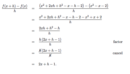
1. To find \(f(x+h)\), we replace every occurrence of \(x\) in the formula \(f(x) = x^2-x-2\) with the quantity \((x+h)\) to get

\[ \begin{array}{rclr} f(x+h) & = & (x+h)^2 - (x+h) -2 & \\ & = & x^2 + 2xh + h^2 - x - h - 2. \end{array} \]

So the difference quotient is

2.To find \(g(x+h)\), we replace every occurrence of \(x\) in the formula \(g(x) = \frac{3}{2x+1}\) with the quantity \((x+h)\) to get

\[ \begin{array}{rclr} g(x+h) & = & \dfrac{3}{2(x+h)+1} & \\ & = & \dfrac{3}{2x+2h+1}, \end{array} \]

which yields

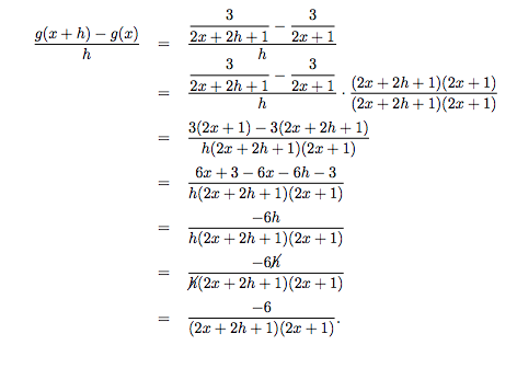
Since we have managed to cancel the original '\(h\)' from the denominator, we are done.

3. For \(r(x) = \sqrt{x}\), we get \(r(x+h) = \sqrt{x+h}\) so the difference quotient is

\[ \dfrac{r(x+h) - r(x)}{h} = \dfrac{\sqrt{x+h} - \sqrt{x}}{h} \]

In order to cancel the '\(h\)' from the denominator, we rationalize the \(\textit{numerator}\) by multiplying by its conjugate.\footnote{Rationalizing the \(\textit{numerator}\)!? How's that for a twist!}

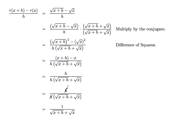
Since we have removed the original '\)h\)' from the denominator, we are done. \(\Box\)

As mentioned before, we will revisit difference quotients in Section 2.1 where we will explain them geometrically. For now, we want to move on to some classic applications of function arithmetic from Economics and for that, we need to think like an entrepreneur.

Suppose you are a manufacturer making a certain product.\footnote{Poorly designed resin Sasquatch statues, for example. Feel free to choose your own entrepreneurial fantasy.} Let \(x\) be the \textbf{production level}, that is, the number of items produced in a given time period. It is customary to let \(C(x)\) denote the function which calculates the total \textbf{cost} of producing the \(x\) items. The quantity \(C(0)\), which represents the cost of producing no items, is called the \(\textbf{fixed}\) cost, and represents the amount of money required to begin production. Associated with the total cost \(C(x)\) is cost per item, or \(\textbf{average cost}\), denoted \(\overline{C}(x)\) and read '\(C\)-bar' of \(x\). To compute \(\overline{C}(x)\), we take the total cost \(C(x)\) and divide by the number of items produced \(x\) to get

\[ \overline{C}(x) = \dfrac{C(x)}{x}\]

On the retail end, we have the \(\textbf{price}\) \(p\) charged per item. To simplify the dialog and computations in this text, we assume that \(\textit{the number of items sold equals the number of items produced}\). From a retail perspective, it seems natural to think of the number of items sold, \(x\), as a function of the price charged, \(p\). After all, the retailer can easily adjust the price to sell more product. In the language of functions, \(x\) would be the \(\textit{dependent}\) variable and \(p\) would be the \(\textit{independent}\) variable or, using function notation, we have a function \(x(p)\). While we will adopt this convention later in the text,\footnote{See Example 5.2.4 in Section 5.2 .} we will hold with tradition at this point and consider the price \(p\) as a function of the number of items sold, \(x\). That is, we regard \(x\) as the independent variable and \(p\) as the dependent variable and speak of the \textbf{price-demand} function, \(p(x)\). Hence, \(p(x)\) returns the price charged per item when \(x\) items are produced and sold. Our next function to consider is the \textbf{revenue} function, \(R(x)\). The function \(R(x)\) computes the amount of money collected as a result of selling \(x\) items. Since \(p(x)\) is the price charged per item, we have \(R(x)= x p(x)\). Finally, the \textbf{profit} function, \(P(x)\) calculates how much money is earned after the costs are paid. That is, \(P(x) = (R-C)(x) = R(x) - C(x)\). We summarize all of these functions below.

Note: Summary of Common Economic Functions

Suppose \(x\) represents the quantity of items produced and sold.

1. The price-demand function \(p(x)\) calculates the price per item.
2. The revenue function \(R(x)\) calculates the total money collected by selling \(x\) items at a price \(p(x)\), \(R(x) = x \, p(x)\).
3. The cost function \(C(x)\) calculates the cost to produce \(x\) items. The value \(C(0)\) is called the fixed cost or start-up cost.
4. The average cost function \(\overline{C}(x) = \frac{C(x)}{x}\) calculates the cost per item when making \(x\) items. Here, we necessarily assume \(x > 0\).
5. The profit function \(P(x)\) calculates the money earned after costs are paid when \(x\) items are produced and sold, \(P(x) = (R-C)(x) = R(x) - C(x)\).

It is high time for an example.

Example \(\PageIndex{1}\): Cost Revenue Profitex

Let \(x\) represent the number of dOpi media players ('dOpis'\footnote{Pronounced 'dopeys' \ldots}) produced and sold in a typical week. Suppose the cost, in dollars, to produce \(x\) dOpis is given by \(C(x) = 100x + 2000\), for \(x \geq 0\), and the price, in dollars per dOpi, is given by \(p(x) = 450-15x\) for \(0 \leq x \leq 30\).

1. Find and interpret \(C(0)\).
2. Find and interpret \(\overline{C}(10)\).
3. Find and interpret \(p(0)\) and \(p(20)\).
4. Solve \(p(x) = 0\) and interpret the result.
5. Find and simplify expressions for the revenue function \(R(x)\) and the profit function \(P(x)\).
6. Find and interpret \(R(0)\) and \(P(0)\).
7. Solve \(P(x) = 0\) and interpret the result.

Solution

1. We substitute \(x=0\) into the formula for \(C(x)\) and get \(C(0) = 100(0) + 2000 = 2000\). This means to produce \(0\) dOpis, it costs \(\\)2000\). In other words, the fixed (or start-up) costs are \(\\)2000\). The reader is encouraged to contemplate what sorts of expenses these might be.
2. Since \(\overline{C}(x) = \frac{C(x)}{x}\), \(\overline{C}(10) = \frac{C(10)}{10} = \frac{3000}{10} = 300\). This means when \(10\) dOpis are produced, the cost to manufacture them amounts to \(\\) 300\) per dOpi.
3. Plugging \(x=0\) into the expression for \(p(x)\) gives \(p(0) = 450 - 15(0) = 450\). This means no dOpis are sold if the price is \(\\)450\) per dOpi. On the other hand, \(p(20) = 450-15(20) = 150\) which means to sell \(20\) dOpis in a typical week, the price should be set at \(\\)150\) per dOpi.
4. Setting \(p(x) = 0\) gives \(450-15x = 0\). Solving gives \(x = 30\). This means in order to sell \(30\) dOpis in a typical week, the price needs to be set to \(\\) 0\). What's more, this means that even if dOpis were given away for free, the retailer would only be able to move \(30\) of them.\footnote{Imagine that! Giving something away for free and hardly anyone taking advantage of it \ldots}
5. To find the revenue, we compute \(R(x) = x p(x) = x (450 - 15x) = 450x - 15x^2\). Since the formula for \(p(x)\) is valid only for \(0 \leq x \leq 30\), our formula \(R(x)\) is also restricted to \(0 \leq x \leq 30\). For the profit, \(P(x) = (R-C)(x) = R(x) - C(x)\). Using the given formula for \(C(x)\) and the derived formula for \(R(x)\), we get \(P(x) = \left(450x - 15x^2\right) -(100x+2000) = -15x^2+350x-2000\). As before, the validity of this formula is for \(0 \leq x \leq 30\) only.
6. We find \(R(0) = 0\) which means if no dOpis are sold, we have no revenue, which makes sense. Turning to profit, \(P(0) = -2000\) since \(P(x) = R(x) - C(x)\) and \(P(0) = R(0) - C(0) = -2000\). This means that if no dOpis are sold, more money (\)\\)2000\) to be exact!) was put into producing the dOpis than was recouped in sales. In number 1, we found the fixed costs to be \(\\)2000\), so it makes sense that if we sell no dOpis, we are out those start-up costs.
7. Setting \(P(x) = 0\) gives \(-15x^2+350x-2000 = 0\). Factoring gives \(-5(x-10)(3x-40) = 0\) so \(x = 10\) or \(x = \frac{40}{3}\). What do these values mean in the context of the problem? Since \(P(x) = R(x) - C(x)\), solving \(P(x) = 0\) is the same as solving \(R(x) = C(x)\). This means that the solutions to \(P(x) = 0\) are the production (and sales) figures for which the sales revenue exactly balances the total production costs. These are the so-called '\textbf{break even}' points. The solution \(x=10\) means \(10\) dOpis should be produced (and sold) during the week to recoup the cost of production. For \(x = \frac{40}{3} = 13.\overline{3}\), things are a bit more complicated. Even though \(x = 13.\overline{3}\) satisfies \(0 \leq x \leq 30\), and hence is in the domain of \(P\), it doesn't make sense in the context of this problem to produce a fractional part of a dOpi.\footnote{We've seen this sort of thing before in Section 1.4 .} Evaluating \(P(13) = 15\) and \(P(14) = -40\), we see that producing and selling \(13\) dOpis per week makes a (slight) profit, whereas producing just one more puts us back into the red. While breaking even is nice, we ultimately would like to find what production level (and price) will result in the largest profit, and we'll do just that \(\ldots\) in Section 2.3 . \(\Box\)