
1.4: Arc Length and Curvature
- Page ID
- 32247
\( \newcommand{\vecs}[1]{\overset { \scriptstyle \rightharpoonup} {\mathbf{#1}} } \)
\( \newcommand{\vecd}[1]{\overset{-\!-\!\rightharpoonup}{\vphantom{a}\smash {#1}}} \)
\( \newcommand{\dsum}{\displaystyle\sum\limits} \)
\( \newcommand{\dint}{\displaystyle\int\limits} \)
\( \newcommand{\dlim}{\displaystyle\lim\limits} \)
\( \newcommand{\id}{\mathrm{id}}\) \( \newcommand{\Span}{\mathrm{span}}\)
( \newcommand{\kernel}{\mathrm{null}\,}\) \( \newcommand{\range}{\mathrm{range}\,}\)
\( \newcommand{\RealPart}{\mathrm{Re}}\) \( \newcommand{\ImaginaryPart}{\mathrm{Im}}\)
\( \newcommand{\Argument}{\mathrm{Arg}}\) \( \newcommand{\norm}[1]{\| #1 \|}\)
\( \newcommand{\inner}[2]{\langle #1, #2 \rangle}\)
\( \newcommand{\Span}{\mathrm{span}}\)
\( \newcommand{\id}{\mathrm{id}}\)
\( \newcommand{\Span}{\mathrm{span}}\)
\( \newcommand{\kernel}{\mathrm{null}\,}\)
\( \newcommand{\range}{\mathrm{range}\,}\)
\( \newcommand{\RealPart}{\mathrm{Re}}\)
\( \newcommand{\ImaginaryPart}{\mathrm{Im}}\)
\( \newcommand{\Argument}{\mathrm{Arg}}\)
\( \newcommand{\norm}[1]{\| #1 \|}\)
\( \newcommand{\inner}[2]{\langle #1, #2 \rangle}\)
\( \newcommand{\Span}{\mathrm{span}}\) \( \newcommand{\AA}{\unicode[.8,0]{x212B}}\)
\( \newcommand{\vectorA}[1]{\vec{#1}} % arrow\)
\( \newcommand{\vectorAt}[1]{\vec{\text{#1}}} % arrow\)
\( \newcommand{\vectorB}[1]{\overset { \scriptstyle \rightharpoonup} {\mathbf{#1}} } \)
\( \newcommand{\vectorC}[1]{\textbf{#1}} \)
\( \newcommand{\vectorD}[1]{\overrightarrow{#1}} \)
\( \newcommand{\vectorDt}[1]{\overrightarrow{\text{#1}}} \)
\( \newcommand{\vectE}[1]{\overset{-\!-\!\rightharpoonup}{\vphantom{a}\smash{\mathbf {#1}}}} \)
\( \newcommand{\vecs}[1]{\overset { \scriptstyle \rightharpoonup} {\mathbf{#1}} } \)
\(\newcommand{\longvect}{\overrightarrow}\)
\( \newcommand{\vecd}[1]{\overset{-\!-\!\rightharpoonup}{\vphantom{a}\smash {#1}}} \)
\(\newcommand{\avec}{\mathbf a}\) \(\newcommand{\bvec}{\mathbf b}\) \(\newcommand{\cvec}{\mathbf c}\) \(\newcommand{\dvec}{\mathbf d}\) \(\newcommand{\dtil}{\widetilde{\mathbf d}}\) \(\newcommand{\evec}{\mathbf e}\) \(\newcommand{\fvec}{\mathbf f}\) \(\newcommand{\nvec}{\mathbf n}\) \(\newcommand{\pvec}{\mathbf p}\) \(\newcommand{\qvec}{\mathbf q}\) \(\newcommand{\svec}{\mathbf s}\) \(\newcommand{\tvec}{\mathbf t}\) \(\newcommand{\uvec}{\mathbf u}\) \(\newcommand{\vvec}{\mathbf v}\) \(\newcommand{\wvec}{\mathbf w}\) \(\newcommand{\xvec}{\mathbf x}\) \(\newcommand{\yvec}{\mathbf y}\) \(\newcommand{\zvec}{\mathbf z}\) \(\newcommand{\rvec}{\mathbf r}\) \(\newcommand{\mvec}{\mathbf m}\) \(\newcommand{\zerovec}{\mathbf 0}\) \(\newcommand{\onevec}{\mathbf 1}\) \(\newcommand{\real}{\mathbb R}\) \(\newcommand{\twovec}[2]{\left[\begin{array}{r}#1 \\ #2 \end{array}\right]}\) \(\newcommand{\ctwovec}[2]{\left[\begin{array}{c}#1 \\ #2 \end{array}\right]}\) \(\newcommand{\threevec}[3]{\left[\begin{array}{r}#1 \\ #2 \\ #3 \end{array}\right]}\) \(\newcommand{\cthreevec}[3]{\left[\begin{array}{c}#1 \\ #2 \\ #3 \end{array}\right]}\) \(\newcommand{\fourvec}[4]{\left[\begin{array}{r}#1 \\ #2 \\ #3 \\ #4 \end{array}\right]}\) \(\newcommand{\cfourvec}[4]{\left[\begin{array}{c}#1 \\ #2 \\ #3 \\ #4 \end{array}\right]}\) \(\newcommand{\fivevec}[5]{\left[\begin{array}{r}#1 \\ #2 \\ #3 \\ #4 \\ #5 \\ \end{array}\right]}\) \(\newcommand{\cfivevec}[5]{\left[\begin{array}{c}#1 \\ #2 \\ #3 \\ #4 \\ #5 \\ \end{array}\right]}\) \(\newcommand{\mattwo}[4]{\left[\begin{array}{rr}#1 \amp #2 \\ #3 \amp #4 \\ \end{array}\right]}\) \(\newcommand{\laspan}[1]{\text{Span}\{#1\}}\) \(\newcommand{\bcal}{\cal B}\) \(\newcommand{\ccal}{\cal C}\) \(\newcommand{\scal}{\cal S}\) \(\newcommand{\wcal}{\cal W}\) \(\newcommand{\ecal}{\cal E}\) \(\newcommand{\coords}[2]{\left\{#1\right\}_{#2}}\) \(\newcommand{\gray}[1]{\color{gray}{#1}}\) \(\newcommand{\lgray}[1]{\color{lightgray}{#1}}\) \(\newcommand{\rank}{\operatorname{rank}}\) \(\newcommand{\row}{\text{Row}}\) \(\newcommand{\col}{\text{Col}}\) \(\renewcommand{\row}{\text{Row}}\) \(\newcommand{\nul}{\text{Nul}}\) \(\newcommand{\var}{\text{Var}}\) \(\newcommand{\corr}{\text{corr}}\) \(\newcommand{\len}[1]{\left|#1\right|}\) \(\newcommand{\bbar}{\overline{\bvec}}\) \(\newcommand{\bhat}{\widehat{\bvec}}\) \(\newcommand{\bperp}{\bvec^\perp}\) \(\newcommand{\xhat}{\widehat{\xvec}}\) \(\newcommand{\vhat}{\widehat{\vvec}}\) \(\newcommand{\uhat}{\widehat{\uvec}}\) \(\newcommand{\what}{\widehat{\wvec}}\) \(\newcommand{\Sighat}{\widehat{\Sigma}}\) \(\newcommand{\lt}{<}\) \(\newcommand{\gt}{>}\) \(\newcommand{\amp}{&}\) \(\definecolor{fillinmathshade}{gray}{0.9}\)In this section, we study formulas related to curves in both two and three dimensions, and see how they are related to various properties of the same curve. For example, suppose a vector-valued function describes the motion of a particle in space. We would like to determine how far the particle has traveled over a given time interval, which can be described by the arc length of the path it follows. Or, suppose that the vector-valued function describes a road we are building and we want to determine how sharply the road curves at a given point. This is described by the curvature of the function at that point. We explore each of these concepts in this section.
Arc Length for Vector Functions
We have seen how a vector-valued function describes a curve in either two or three dimensions. Recall that the formula for the arc length of a curve defined by the parametric functions \(x=x(t)\) and \(y=y(t)\), for \(t_1≤t≤t_2\) is given by
\[s=\int^{t_2}_{t_1} \sqrt{(x^{\,\prime}(t))^2+(y^{\,\prime}(t))^2}\,dt.\]
In a similar fashion, if we define a smooth curve using a vector-valued function \(\vecs r(t)=f(t) \,\hat{\mathbf{i}}+g(t) \,\hat{\mathbf{j}}\), where \(a≤t≤b\), the arc length is given by the formula
\[s=\int^{b}_{a} \sqrt{(f^{\,\prime}(t))^2+(g^{\,\prime}(t))^2}\,dt.\]
In three dimensions, if the vector-valued function is described by \(\vecs r(t)=f(t) \,\hat{\mathbf{i}}+g(t) \,\hat{\mathbf{j}}+h(t) \,\hat{\mathbf{k}}\) over the same interval \(a≤t≤b\), the arc length is given by
\[s=\int^{b}_{a} \sqrt{(f^{\,\prime}(t))^2+(g^{\,\prime}(t))^2+(h^{\,\prime}(t))^2}\,dt.\]
Theorem: Arc-Length Formulas for Plane and Space curves
Plane curve: Given a smooth curve \(C\) defined by the function \(\vecs r(t)=f(t) \,\hat{\mathbf{i}}+g(t) \, \hat{\mathbf{j}}\), where \(t\) lies within the interval \([a,b]\), the arc length of \(C\) over the interval is
\[\begin{align} s&=\int^{b}_{a} \sqrt{[f^{\,\prime}(t)]^2+[g^{\,\prime}(t)]^2}\,dt \\[5pt] &=\int^{b}_{a} \|\vecs r^{\,\prime}(t)\|\,dt . \label{Arc2D}\end{align}\]
Space curve: Given a smooth curve \(C\) defined by the function \(\vecs r(t)=f(t) \,\hat{\mathbf{i}}+g(t) \,\hat{\mathbf{j}}+h(t) \,\hat{\mathbf{k}}\), where \(t\) lies within the interval \([a,b]\), the arc length of \(C\) over the interval is
\[\begin{align} s&=\int^{b}_{a} \sqrt{[f^{\,\prime}(t)]^2+[g^{\,\prime}(t)]^2+[h^{\,\prime}(t)]^2}\,dt \\[5pt] &=\int^{b}_{a} \|\vecs r^{\,\prime}(t)\|\,dt . \label{Arc3D} \end{align}\]
The two formulas are very similar; they differ only in the fact that a space curve has three component functions instead of two. Note that the formulas are defined for smooth curves: curves where the vector-valued function \(\vecs r(t)\) is differentiable with a non-zero derivative. The smoothness condition guarantees that the curve has no cusps (or corners) that could make the formula problematic.
Example \(\PageIndex{1}\): Finding the Arc Length
Calculate the arc length for each of the following vector-valued functions:
- \(\vecs r(t)=(3t−2) \,\hat{\mathbf{i}}+(4t+5) \,\hat{\mathbf{j}},\quad 1≤t≤5\)
- \(\vecs r(t)=⟨t\cos t,t\sin t,2t⟩,0≤t≤2 \pi \)
Solution
- Using Equation \ref{Arc2D}, \(\vecs r^{\,\prime}(t)=3 \,\hat{\mathbf{i}}+4 \,\hat{\mathbf{j}}\), so
\[\begin{align*} s \; & =\int^{b}_{a} \|\vecs r^{\,\prime}(t)\|\,dt \\ & =\int^{5}_{1} \sqrt{3^2 + 4^2} \,dt \\[5pt] & =\int^{5}_{1} 5 \,dt = 5t\big|^{5}_{1} = 20. \end{align*}\]
- Using Equation \ref{Arc3D}, \(\vecs r^{\,\prime}(t)=⟨ \cos t−t \sin t, \sin t+t \cos t,2⟩ \), so
\[\begin{align*} s \; & =\int^{b}_{a} ∥\vecs r^{\,\prime}(t)∥\,dt \\ & =\int^{2 \pi}_{0} \sqrt{(\cos t−t \sin t)^2+( \sin t+t \cos t)^2+2^2} \,dt \\[5pt] & =\int^{2 \pi}_{0} \sqrt{( \cos ^2 t−2t \sin t \cos t+t^2 \sin ^2 t)+( \sin^2 t+2t \sin t \cos t+t^2 \cos ^2 t)+4} \,dt \\ & =\int^{2 \pi}_{0} \sqrt{\cos ^2 t+ \sin^2 t+t^2( \cos ^2 t+ \sin ^2 t)+4} \,dt \\[5pt] & =\int^{2 \pi}_{0} \sqrt{t^2+5} \,dt\end{align*}\]
Here we can use a table integration formula
\[\int \sqrt{u^2+a^2}du = \dfrac{u}{2}\sqrt{u^2+a^2} + \dfrac{a^2}{2} \ln \,\left|\, u + \sqrt{u^2+a^2} \,\right| + C, \nonumber\]
so we obtain
\[\begin{align*} \int^{2 \pi}_{0} \sqrt{t^2+5} \,dt \; & = \frac{1}{2} \bigg( t \sqrt{t^2+5}+5 \ln \,\left|t+\sqrt{t^2+5}\right| \bigg) _0^{2π} \\[5pt] & = \frac{1}{2} \bigg( 2π \sqrt{4π^2+5}+5 \ln \bigg( 2π+ \sqrt{4π^2+5} \bigg) \bigg)−\frac{5}{2} \ln \sqrt{5} \\[5pt] & ≈25.343 \,\text{units}. \end{align*}\]
Exercise \(\PageIndex{1}\)
Calculate the arc length of the parameterized curve
\[\vecs r(t)=⟨2t^2+1,2t^2−1,t^3⟩,\quad 0≤t≤3. \nonumber\]
- Hint
-
Use Equation \ref{Arc3D}.
- Answer
-
\(\vecs r^{\,\prime}(t)=⟨4t,4t,3t^2⟩,\) so \(s= \frac{1}{27}(113^{3/2}−32^{3/2})≈37.785\) units
We now return to the helix introduced earlier in this chapter. A vector-valued function that describes a helix can be written in the form
\[\vecs r(t)=R \cos \left(\dfrac{2πNt}{h}\right) \,\hat{\mathbf{i}} +R \sin \left(\dfrac{2πNt}{h}\right) \,\hat{\mathbf{j}}+t \,\hat{\mathbf{k}},0≤t≤h,\]
where \(R\) represents the radius of the helix, \(h\) represents the height (distance between two consecutive turns), and the helix completes \(N\) turns. Let’s derive a formula for the arc length of this helix using Equation \ref{Arc3D}. First of all,
\[\vecs r^{\,\prime}(t)=−\dfrac{2πNR}{h} \sin \left(\dfrac{2πNt}{h}\right) \,\hat{\mathbf{i}}+ \dfrac{2πNR}{h} \cos \left(\dfrac{2πNt}{h} \right) \,\hat{\mathbf{j}}+\,\hat{\mathbf{k}}.\]
Therefore,
\[\begin{align} s \; & =\int_a^b ‖\vecs r^{\,\prime}(t)‖\,dt \\[5pt]
&=\int_0^h\sqrt{ \bigg(−\dfrac{2πNR}{h} \sin \bigg(\dfrac{2πNt}{h} \bigg) \bigg)^2+ \bigg( \dfrac{2πNR}{h} \cos \bigg( \dfrac{2πNt}{h} \bigg) \bigg)^2+1^2}\,dt \\[5pt]
&=\int_0^h\sqrt{ \dfrac{4π^2N^2R^2}{h^2} \bigg( \sin ^2 \bigg(\dfrac{2πNt}{h} \bigg) + \cos ^2 \bigg( \dfrac{2πNt}{h} \bigg) \bigg)+1}\,dt \\[5pt]
&=\int_0^h\sqrt{ \dfrac{4π^2N^2R^2}{h^2} +1}\,dt \\[5pt]
&=\bigg[ t\sqrt{ \dfrac{4π^2N^2R^2}{h^2} +1}\bigg]^h_0 \\[5pt]
&=h \sqrt{ \dfrac{4π^2N^2R^2 + h^2}{h^2}} \\[5pt]
&=\sqrt{ 4π^2N^2R^2 + h^2}.\end{align}\]
This gives a formula for the length of a wire needed to form a helix with \(N\) turns that has radius \(R\) and height \(h\).
Arc-Length Parameterization
We now have a formula for the arc length of a curve defined by a vector-valued function. Let’s take this one step further and examine what an arc-length function is.
If a vector-valued function represents the position of a particle in space as a function of time, then the arc-length function measures how far that particle travels as a function of time. The formula for the arc-length function follows directly from the formula for arc length:
\[s=\int^{t}_{a} \sqrt{(f^{\,\prime}(u))^2+(g^{\,\prime}(u))^2+(h^{\,\prime}(u))^2}du. \label{arclength2}\]
If the curve is in two dimensions, then only two terms appear under the square root inside the integral. The reason for using the independent variable u is to distinguish between time and the variable of integration. Since \(s(t)\) measures distance traveled as a function of time, \(s^{\,\prime}(t)\) measures the speed of the particle at any given time. Since we have a formula for \(s(t)\) in Equation \ref{arclength2}, we can differentiate both sides of the equation:
\[ \begin{align} s^{\,\prime}(t) \; & =\dfrac{d}{\,dt} \bigg[ \int^{t}_{a} \sqrt{(f^{\,\prime}(u))^2+(g^{\,\prime}(u))^2+(h^{\,\prime}(u))^2}du \bigg] \\[5pt]
&=\dfrac{d}{\,dt} \bigg[ \int^{t}_{a} ‖\vecs r^{\,\prime}(u)‖du \bigg] \\[5pt]
&=\|\vecs r^{\,\prime}(t)\|.\end{align}\]
If we assume that \(\vecs r(t)\) defines a smooth curve, then the arc length is always increasing, so \(s^{\,\prime}(t)>0\) for \(t>a\). Last, if \(\vecs r(t)\) is a curve on which \(\|\vecs r^{\,\prime}(t)\|=1 \) for all \(t\), then
\[s(t)=\int^{t}_{a} ‖\vecs r^{\,\prime}(u)‖\,du=\int^{t}_{a} 1\,du=t−a,\]
which means that \(t\) represents the arc length as long as \(a=0\).
Theorem: Arc-Length Function
Let \(\vecs r(t)\) describe a smooth curve for \(t≥a\). Then the arc-length function is given by
\[s(t)=\int^{t}_{a} ‖\vecs r^{\,\prime}(u)‖\,du\]
Furthermore, \(\frac{ds}{\,dt}=‖\vecs r^{\,\prime}(t)‖>0.\) If \(‖\vecs r^{\,\prime}(t)‖=1\) for all \(t≥a\), then the parameter \(t\) represents the arc length from the starting point at \(t=a\).
A useful application of this theorem is to find an alternative parameterization of a given curve, called an arc-length parameterization. Recall that any vector-valued function can be reparameterized via a change of variables. For example, if we have a function \(\vecs r(t)=⟨3 \cos t,3 \sin t⟩,0≤t≤2π\) that parameterizes a circle of radius 3, we can change the parameter from \(t\) to \(4t\), obtaining a new parameterization \(\vecs r(t)=⟨3 \cos 4t,3 \sin 4t⟩\). The new parameterization still defines a circle of radius 3, but now we need only use the values \(0≤t≤π/2\) to traverse the circle once.
Suppose that we find the arc-length function \(s(t)\) and are able to solve this function for \(t\) as a function of \(s\). We can then reparameterize the original function \(\vecs r(t)\) by substituting the expression for \(t\) back into \(\vecs r(t)\). The vector-valued function is now written in terms of the parameter \(s\). Since the variable \(s\) represents the arc length, we call this an arc-length parameterization of the original function \(\vecs r(t)\). One advantage of finding the arc-length parameterization is that the distance traveled along the curve starting from \(s=0\) is now equal to the parameter \(s\). The arc-length parameterization also appears in the context of curvature (which we examine later in this section) and line integrals.
Example \(\PageIndex{2}\): Finding an Arc-Length Parameterization
Find the arc-length parameterization for each of the following curves:
- \(\vecs r(t)=4 \cos t \,\hat{\mathbf{i}}+ 4 \sin t \,\hat{\mathbf{j}},\quad t≥0\)
- \(\vecs r(t)=⟨t+3,2t−4,2t⟩,\quad t≥3\)
Solution
- First we find the arc-length function using Equation \ref{arclength2}:
\[\begin{align*} s(t) \; & = \int_a^t ‖\vecs r^{\,\prime}(u)‖ \,du \\[5pt]
&= \int_0^t ‖⟨−4 \sin u,4 \cos u⟩‖ \,du \\[5pt]
&= \int_0^t \sqrt{(−4 \sin u)^2+(4 \cos u)^2} \,du \\[5pt]
&= \int_0^t \sqrt{16 \sin ^2 u+16 \cos ^2 u} \,du \\[5pt]
&= \int_0^t 4\,du = 4t, \end{align*}\]which gives the relationship between the arc length \(s\) and the parameter \(t\) as \(s=4t;\) so, \(t=s/4\). Next we replace the variable \(t\) in the original function \(\vecs r(t)=4 \cos t \,\hat{\mathbf{i}}+4 \sin t \,\hat{\mathbf{j}}\) with the expression \(s/4\) to obtain
\[\vecs r(s)=4 \cos \left(\frac{s}{4}\right) \,\hat{\mathbf{i}} + 4 \sin \left( \frac{s}{4}\right) \,\hat{\mathbf{j}}. \nonumber\]
This is the arc-length parameterization of \(\vecs r(t)\). Since the original restriction on \(t\) was given by \(t≥0\), the restriction on s becomes \(s/4≥0\), or \(s≥0\). - The arc-length function is given by Equation \ref{arclength2}:
\[\begin{align*} s(t) \; & = \int_a^t ‖\vecs r^{\,\prime}(u)‖ \,du \\[5pt]
Therefore, the relationship between the arc length \(s\) and the parameter \(t\) is \(s=3t−9\), so \(t= \frac{s}{3}+3\). Substituting this into the original function \(\vecs r(t)=⟨t+3,2t−4,2t⟩ \) yields
&= \int_3^t ‖⟨1,2,2⟩‖ \,du \\[5pt]
&= \int_3^t \sqrt{1^2+2^2+2^2} \,du \\[5pt]
&= \int_3^t 3 \,du \\[5pt]
&= 3t - 9. \end{align*}\]\[\vecs r(s)=⟨\left(\frac{s}{3}+3\right)+3,\,2\left(\frac{s}{3}+3\right)−4,\,2\left(\frac{s}{3}+3\right)⟩=⟨\frac{s}{3}+6, \frac{2s}{3}+2,\frac{2s}{3}+6⟩.\nonumber\]
This is an arc-length parameterization of \(\vecs r(t)\). The original restriction on the parameter \(t\) was \(t≥3\), so the restriction on s is \((s/3)+3≥3\), or \(s≥0\).
Exercise \(\PageIndex{2}\)
Find the arc-length function for the helix
\[\vecs r(t)=⟨3 \cos t, 3 \sin t,4t⟩,\quad t≥0. \nonumber\]
Then, use the relationship between the arc length and the parameter \(t\) to find an arc-length parameterization of \(\vecs r(t)\).
- Hint
-
Start by finding the arc-length function.
- Answer
-
\(s=5t\), or \(t=s/5\). Substituting this into \(\vecs r(t)=⟨3 \cos t,3 \sin t,4t⟩\) gives
\(\vecs r(s)=⟨3 \cos \left(\frac{s}{5}\right),3 \sin \left(\frac{s}{5}\right),\frac{4s}{5}⟩,\quad s≥0\).
Curvature
An important topic related to arc length is curvature. The concept of curvature provides a way to measure how sharply a smooth curve turns. A circle has constant curvature. The smaller the radius of the circle, the greater the curvature.
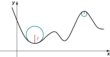
Think of driving down a road. Suppose the road lies on an arc of a large circle. In this case you would barely have to turn the wheel to stay on the road. Now suppose the radius is smaller. In this case you would need to turn more sharply to stay on the road. In the case of a curve other than a circle, it is often useful first to inscribe a circle to the curve at a given point so that it is tangent to the curve at that point and “hugs” the curve as closely as possible in a neighborhood of the point (Figure \(\PageIndex{1}\)). The curvature of the graph at that point is then defined to be the same as the curvature of the inscribed circle.
Definition: curvature
Let \(C\) be a smooth curve in the plane or in space given by \(\vecs r(s)\), where \(s\) is the arc-length parameter. The curvature \(κ\) at \(s\) is
\[κ =\bigg{\|}\dfrac{d\vecs{T}}{ds}\bigg{\|}=‖\vecs T^{\,\prime}(s)‖.\]
As the unit vector \(\vecs T(t)\) is not changing in length, the curvature could be described as a measure of the speed at which the direction of the motion is changing. Since the parameter here is \(s\), we have forced the varying speed of travel along the path out of this measurement.
The formula in the definition of curvature is not very useful in terms of calculation. In particular, recall that \(\vecs T(t)\) represents the unit tangent vector to a given vector-valued function \(\vecs r(t)\), and the formula for \(\vecs T(t)\) is
\[\vecs T(t)=\frac{\vecs r^{\,\prime}(t)}{∥\vecs r^{\,\prime}(t)∥}.\]
To use the formula for curvature, it is first necessary to express \(\vecs r(t)\) in terms of the arc-length parameter \(s\), then find the unit tangent vector \(\vecs T(s)\) for the function \(\vecs r(s)\), then take the derivative of \(\vecs T(s)\) with respect to \(s\). This is a tedious process. Fortunately, there are equivalent formulas for curvature.
Theorem: Alternate Formulas of Curvature
If \(C\) is a smooth curve given by \(\vecs r(t)\), then the curvature \(κ\) of \(C\) at \(t\) is given by
\[κ =\dfrac{‖\vecs T^{\,\prime}(t)‖}{‖\vecs r^{\,\prime}(t)‖}. \label{EqK2}\]
If \(C\) is a three-dimensional curve, then the curvature can be given by the formula
\[κ =\dfrac{‖\vecs r^{\,\prime}(t)×\vecs r′^{\,\prime}(t)‖}{‖\vecs r^{\,\prime}(t)‖^3}.\label{EqK3}\]
Note that in the context of motion, this formula could also be written
\[κ =\dfrac{‖\vecs v(t)×\vecs a(t)‖}{‖\vecs v(t)‖^3}.\nonumber\]
If \(C\) is the graph of a function \(y=f(x)\) and both \(y^{\,\prime}\) and \(y^{\,\prime\prime}\) exist, then the curvature \(κ\) at point \((x,y)\) is given by
\[κ =\dfrac{\big|y^{\,\prime\prime}\big|}{\big[1+\left(y^{\,\prime}\right)^2\big]^{3/2}}.\label{EqK4}\]
Proof
The first formula follows directly from the chain rule:
\[\dfrac{d\vecs{T}}{\,dt} = \dfrac{d\vecs{T}}{ds} \dfrac{ds}{\,dt}, \nonumber\]
where \(s\) is the arc length along the curve \(C\). Dividing both sides by \(ds/\,dt\), and taking the magnitude of both sides gives
\[\bigg{\|}\dfrac{d\vecs{T}}{ds}\bigg{\|}= \left\lVert\frac{\vecs T^{\,\prime}(t)}{\dfrac{ds}{\,dt}}\right\rVert.\nonumber\]
Since \(ds/\,dt=‖\vecs r^{\,\prime}(t)‖\), this gives the formula for the curvature \(κ\) of a curve \(C\) in terms of any parameterization of \(C\):
\[κ =\dfrac{‖\vecs T^{\,\prime}(t)‖}{‖\vecs r^{\,\prime}(t)‖}.\nonumber\]
In the case of a three-dimensional curve, we start with the formulas \(\vecs T(t)=(\vecs r^{\,\prime}(t))/‖\vecs r^{\,\prime}(t)‖\) and \(ds/\,dt=‖\vecs r^{\,\prime}(t)‖\). Therefore, \(\vecs r^{\,\prime}(t)=(ds/\,dt)\vecs T(t)\). We can take the derivative of this function using the scalar product formula:
\[\vecs r^{\,\prime\prime}(t)=\dfrac{d^2s}{\,dt^2}\vecs T(t)+\dfrac{ds}{\,dt}\vecs T^{\,\prime}(t).\nonumber\]
Using these last two equations we get
\[\begin{align*} \vecs r^{\,\prime}(t)×\vecs r^{\,\prime\prime}(t) \; & =\dfrac{ds}{\,dt}\vecs T(t)× \bigg( \dfrac{d^2s}{\,dt^2}\vecs T(t)+\dfrac{ds}{\,dt}\vecs T^{\,\prime}(t) \bigg) \\ & =\dfrac{ds}{\,dt} \dfrac{d^2s}{\,dt^2}\vecs T(t)×\vecs T(t)+(\dfrac{ds}{\,dt})^2\vecs T(t)×\vecs T^{\,\prime}(t). \end{align*}\]
Since \(\vecs T(t)×\vecs T(t)=0\), this reduces to
\[\vecs r^{\,\prime}(t)×\vecs r′^{\,\prime}(t)=\left(\dfrac{ds}{\,dt}\right)^2\vecs T(t)×\vecs T^{\,\prime}(t).\nonumber\]
Since \(\vecs T′\) is parallel to \(\vecs N\), and \(\vecs T\) is orthogonal to \(\vecs N\), it follows that \(\vecs T\) and \(\vecs T′\) are orthogonal. This means that \(‖\vecs T×\vecs T′‖=‖\vecs T‖‖\vecs T′‖ \sin (π/2)=‖\vecs T′‖\), so
\[\|\vecs r^{\,\prime}(t)×\vecs r^{\,\prime\prime}(t)\|=\left(\dfrac{ds}{\,dt}\right)^2‖\vecs T^{\,\prime}(t)‖.\nonumber\]
Now we solve this equation for \(‖\vecs T^{\,\prime}(t)‖\) and use the fact that \(ds/\,dt=‖\vecs r^{\,\prime}(t)‖\):
\[‖\vecs T^{\,\prime}(t)‖=\dfrac{‖\vecs r^{\,\prime}(t)×\vecs r^{\,\prime\prime}(t)‖}{‖\vecs r^{\,\prime}(t)‖^2}.\nonumber\]
Then, we divide both sides by \(‖\vecs r^{\,\prime}(t)‖\). This gives
\[κ =\dfrac{‖\vecs T^{\,\prime}(t)‖}{‖\vecs r^{\,\prime}(t)‖}=\dfrac{‖\vecs r^{\,\prime}(t)×\vecs r^{\,\prime\prime}(t)‖}{‖\vecs r^{\,\prime}(t)‖^3}.\nonumber\]
This proves \(\ref{EqK3}\). To prove \(\ref{EqK4}\), we start with the assumption that curve \(C\) is defined by the function \(y=f(x)\). Then, we can define \(\vecs r(t)=x \,\hat{\mathbf{i}}+f(x) \,\hat{\mathbf{j}}+0 \,\hat{\mathbf{k}}\). Using the previous formula for curvature:
\[\begin{align*} \vecs r^{\,\prime}(t) \; & =\,\hat{\mathbf{i}}+f^{\,\prime}(x)\,\hat{\mathbf{j}} \\[5pt] \vecs r^{\,\prime\prime}(t) \; & =f^{\,\prime\prime}(x)\,\hat{\mathbf{j}} \\[5pt] \vecs r^{\,\prime}(t)×\vecs r^{\,\prime\prime}(t) \; & = \begin{vmatrix}\hat{\mathbf{i}} &\,\hat{\mathbf{j}} &\,\hat{\mathbf{k}} \\ 1 & f^{\,\prime}(x) & 0 \\ 0 & f^{\,\prime\prime}(x) & 0 \end{vmatrix} =f^{\,\prime\prime}(x)\,\hat{\mathbf{k}}. \end{align*}\]
Therefore,
\[κ= \dfrac{‖\vecs r^{\,\prime}(t)×\vecs r^{\,\prime\prime}(t)‖}{‖\vecs r^{\,\prime}(t)‖^3}=\dfrac{|f^{\,\prime\prime}(x)|}{(1+[f^{\,\prime}(x)]^2)^{3/2}} \nonumber\]
Note that in the context of motion, the first alternate formula can be rewritten
\[κ =\dfrac{‖\vecs T^{\,\prime}(t)‖}{‖\vecs v(t)‖}.\]
Considering what was stated above about the curvature being a measure of the speed at which the direction of motion is changing at a point, notice that we have normalized this measurement this time by dividing out the actual speed of travel along the curve at the given instant.
As indicated above, the second alternate formula can be rewritten as
\[κ =\dfrac{‖\vecs v(t)×\vecs a(t)‖}{‖\vecs v(t)‖^3}.\]
Remember that the cross product measures the extent to which the two vectors are aligned, returning its largest value when they are orthogonal. Note also that the component of acceleration that is orthogonal to the velocity is the only part we care about here, as it is the component that will affect the change of direction of the motion. The component of acceleration that is aligned with the velocity (and tangent to the curve) will only affect the speed of the motion, which is being ignored in our measurement of curvature. Note that one factor of \(\frac{1}{‖\vecs v(t)‖}\) will multiply into the cross product to make the first vector be \(\vecs T(t)\).
Example \(\PageIndex{3}\): Finding Curvature
Find the curvature for each of the following curves at the given point:
- \(\vecs r(t)=4 \cos t\,\hat{\mathbf{i}}+4 \sin t\,\hat{\mathbf{j}}+3t\,\hat{\mathbf{k}},\quad t=\dfrac{4π}{3}\)
- \(f(x)= \sqrt{4x−x^2},\quad x=2\)
Solution
- This function describes a helix.
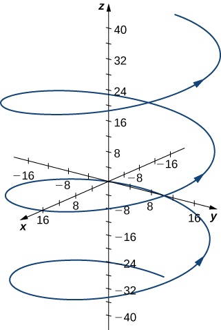
The curvature of the helix at \(t=(4π)/3\) can be found by using \(\ref{EqK2}\). First, calculate \(\vecs T(t)\):
\[\begin{align*} \vecs T(t) \; & =\dfrac{\vecs r^{\,\prime}(t)}{‖\vecs r^{\,\prime}(t)‖} \\[5pt] & =\dfrac{⟨−4 \sin t,4 \cos t,3⟩}{\sqrt{(−4 \sin t)^2+(4 \cos t)^2+3^2}}\\[5pt] & =⟨−\dfrac{4}{5} \sin t,\dfrac{4}{5} \cos t, \dfrac{3}{5}⟩. \end{align*}\]
Next, calculate \(\vecs T^{\,\prime}(t):\)
\[\vecs T^{\,\prime}(t)=⟨−\dfrac{4}{5} \cos t,− \dfrac{4}{5} \sin t,0⟩. \nonumber\]
Last, apply \(\ref{EqK2}\):
\[ \begin{align*} κ \; &=\dfrac{‖\vecs T^{\,\prime}(t)‖}{‖\vecs r^{\,\prime}(t)‖} = \dfrac{‖⟨−\dfrac{4}{5} \cos t,−\dfrac{4}{5} \sin t,0⟩‖}{‖⟨−4 \sin t,4 \cos t,3⟩‖} \\[5pt] & =\dfrac{\sqrt{(−\dfrac{4}{5} \cos t)^2+(−\dfrac{4}{5} \sin t)^2+0^2}}{\sqrt{(−4 \sin t)^2+(4 \cos t)^2+ 3^2}} \\[5pt] & =\dfrac{4/5}{5}=\dfrac{4}{25}. \end{align*}\]
The curvature of this helix is constant at all points on the helix.
- This function describes a semicircle.
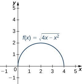
To find the curvature of this graph, we must use \(\ref{EqK4}\). First, we calculate \(y^{\,\prime}\) and \(y^{\,\prime\prime}:\)
\[\begin{align*}y \; &=\sqrt{4x−x^2}=(4x−x^2)^{1/2} \\[5pt] y^{\,\prime} \; &=\dfrac{1}{2}(4x−x^2)^{−1/2}(4−2x)=(2−x)(4x−x^2)^{−1/2} \\[5pt] y^{\,\prime\prime} \; &=−(4x−x^2)^{−1/2}+(2−x)(−\dfrac{1}{2})(4x−x^2)^{−3/2}(4−2x) \\[5pt] &=−\dfrac{4x−x^2}{(4x−x^2)^{3/2}}− \dfrac{(2−x)^2}{(4x−x^2)^{3/2}} \\[5pt] &=\dfrac{x^2−4x−(4−4x+x^2)}{(4x−x^2)^{3/2}} \\[5pt] & =−\dfrac{4}{(4x−x^2)^{3/2}}. \end{align*} \]
Then, we apply \(\ref{EqK4}\):
\[ \begin{align*} κ \; &=\dfrac{|y^{\,\prime\prime}|}{[1+(y^{\,\prime})^2]^{3/2}} \\[5pt]
&= \dfrac{\bigg| −\dfrac{4}{(4x−x^2)^{3/2}}\bigg|}{\bigg[1+((2−x)(4x−x^2)^{−1/2})^2 \bigg]^{3/2}} = \dfrac{\bigg| \dfrac{4}{(4x−x^2)^{3/2}} \bigg|}{\bigg[ 1+\dfrac{(2−x)^2}{4x−x^2} \bigg]^ {3/2}} \\[5pt]
&= \dfrac{\bigg| \dfrac{4}{(4x−x^2)^{3/2}} \bigg|}{ \bigg[ \dfrac{4x−x^2+x^2−4x+4}{4x−x^2} \bigg]^{3/2}}=\bigg| \dfrac{4}{(4x−x^2)^{3/2}} \bigg| ⋅\dfrac{(4x−x^2)^{3/2}}{8} \\[5pt]
&=\dfrac{1}{2}. \end{align*}\]
The curvature of this circle is equal to the reciprocal of its radius. There is a minor issue with the absolute value in \(\ref{EqK4}\); however, a closer look at the calculation reveals that the denominator is positive for any value of \(x\).
Exercise \(\PageIndex{3}\)
Find the curvature of the curve defined by the function
\[y=3x^2−2x+4 \nonumber\]
at the point \(x=2\).
- Hint
-
Use \(\ref{EqK4}\).
- Answer
-
\(κ \; =\frac{6}{101^{3/2}}≈0.0059\)
The Normal and Binormal Vectors
We have seen that the derivative \(\vecs r^{\,\prime}(t)\) of a vector-valued function is a tangent vector to the curve defined by \(\vecs r(t)\), and the unit tangent vector \(\vecs T(t)\) can be calculated by dividing \(\vecs r^{\,\prime}(t)\) by its magnitude. When studying motion in three dimensions, two other vectors are useful in describing the motion of a particle along a path in space: the principal unit normal vector and the binormal vector.
Definition: Binormal Vectors
Let \(C\) be a three-dimensional smooth curve represented by \(\vecs r\) over an open interval \(I\). If \(\vecs T^{\,\prime}(t)≠\vecs 0\), then the principal unit normal vector at \(t\) is defined to be
\[\vecs N(t)=\dfrac{\vecs T^{\,\prime}(t)}{‖\vecs T^{\,\prime}(t)‖}. \label{EqNormal}\]
The binormal vector at \(t\) is defined as
\[\vecs B(t)=\vecs T(t)×\vecs N(t), \label{EqBinormal}\]
where \(\vecs T(t)\) is the unit tangent vector.
Note that, by definition, the binormal vector is orthogonal to both the unit tangent vector and the normal vector. Furthermore, \(\vecs B(t)\) is always a unit vector. This can be shown using the formula for the magnitude of a cross product:
\[‖\vecs B(t)‖=‖\vecs T(t)×\vecs N(t)‖=‖\vecs T(t)‖‖\vecs N(t)‖ \sin \theta,\]
where \(\theta\) is the angle between \(\vecs T(t)\) and \(\vecs N(t)\). Since \(\vecs N(t)\) is the derivative of a unit vector, property (vii) of the derivative of a vector-valued function tells us that \(\vecs T(t)\) and \(\vecs N(t)\) are orthogonal to each other, so \(\theta=π/2\). Furthermore, they are both unit vectors, so their magnitude is 1. Therefore, \(‖\vecs T(t)‖‖\vecs N(t)‖ \sin \theta=(1)(1) \sin (π/2)=1\) and \(\vecs B(t)\) is a unit vector.
The principal unit normal vector can be challenging to calculate because the unit tangent vector involves a quotient, and this quotient often has a square root in the denominator. In the three-dimensional case, finding the cross product of the unit tangent vector and the unit normal vector can be even more cumbersome. Fortunately, we have alternative formulas for finding these two vectors, and they are presented in Motion in Space.
Example \(\PageIndex{4}\): Finding the Principal Unit Normal Vector and Binormal Vector
For each of the following vector-valued functions, find the principal unit normal vector. Then, if possible, find the binormal vector.
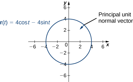
- \(\vecs r(t)=4 \cos t\,\hat{\mathbf{i}}− 4 \sin t\,\hat{\mathbf{j}}\)
- \(\vecs r(t)=(6t+2)\,\hat{\mathbf{i}}+5t^2\,\hat{\mathbf{j}}−8t\,\hat{\mathbf{k}}\)
Solution
- This function describes a circle.
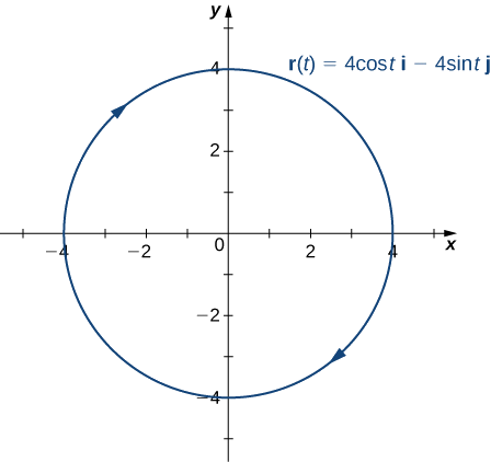
To find the principal unit normal vector, we first must find the unit tangent vector \(\vecs T(t):\)
\[\begin{align*} \vecs T(t) \; &=\dfrac{\vecs r^{\,\prime}(t)}{‖\vecs r^{\,\prime}(t)‖} \\[5pt]
&=\dfrac{−4 \sin t\,\hat{\mathbf{i}}−4 \cos t\,\hat{\mathbf{j}}}{\sqrt{(−4 \sin t)^2+(−4\cos t)^2}} \\[5pt]
&=\dfrac{−4 \sin t\,\hat{\mathbf{i}}−4 \cos t\,\hat{\mathbf{j}} }{\sqrt{16 \sin ^2 t+16 \cos ^2 t}} \\[5pt]
&=\dfrac{−4 \sin t\,\hat{\mathbf{i}}−4 \cos t\,\hat{\mathbf{j}} }{\sqrt{16(\sin ^2 t+ \cos ^2 t)}} \\[5pt]
&=\dfrac{−4 \sin t\,\hat{\mathbf{i}}−4 \cos t\,\hat{\mathbf{j}}}{4} \\[5pt]
&=− \sin t\,\hat{\mathbf{i}}− \cos t\,\hat{\mathbf{j}}.\end{align*}\]
Next, we use \(\ref{EqNormal}\):
\[\begin{align*} \vecs N(t) \; &=\dfrac{\vecs T^{\,\prime}(t)}{‖\vecs T^{\,\prime}(t)‖} \\[5pt]
&=\dfrac{− \cos t\,\hat{\mathbf{i}}+\sin t\,\hat{\mathbf{j}}}{\sqrt{(− \cos t)^2+(\sin t)^2}} \\[5pt]
&=\dfrac{− \cos t\,\hat{\mathbf{i}}+ \sin t\,\hat{\mathbf{j}}}{\sqrt{ \cos ^2 t+ \sin ^2 t}} \\[5pt]
&=− \cos t\,\hat{\mathbf{i}}+ \sin t\,\hat{\mathbf{j}}. \end{align*}\]
Notice that the unit tangent vector and the principal unit normal vector are orthogonal to each other for all values of \(t\):
\[\begin{align*} \vecs T(t)·\vecs N(t) \; &=⟨− \sin t,− \cos t⟩·⟨− \cos t, \sin t⟩ \\ &= \sin t \cos t−\cos t \sin t \\ &=0. \end{align*}\]
Furthermore, the principal unit normal vector points toward the center of the circle from every point on the circle. Since \(\vecs r(t)\) defines a curve in two dimensions, we cannot calculate the binormal vector.
- This function looks like this:
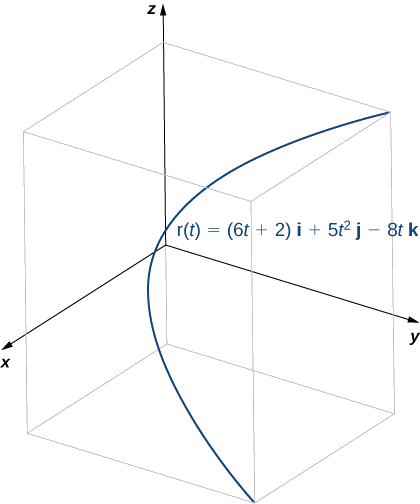
To find the principal unit normal vector, we first find the unit tangent vector \(\vecs T(t):\)
\[\begin{align*} \vecs T(t) \; &=\dfrac{\vecs r^{\,\prime}(t)}{‖\vecs r^{\,\prime}(t)‖} \\[5pt]
&=\dfrac{6\,\hat{\mathbf{i}}+10t\,\hat{\mathbf{j}}−8\,\hat{\mathbf{k}}}{ \sqrt{6^2+(10t)^2+(−8)^2}} \\[5pt]
&=\dfrac{6\,\hat{\mathbf{i}}+10t\,\hat{\mathbf{j}}−8\,\hat{\mathbf{k}}}{ \sqrt{36+100t^2+64}} \\[5pt]
&= \dfrac{6\,\hat{\mathbf{i}}+10t\,\hat{\mathbf{j}}−8\,\hat{\mathbf{k}}}{\sqrt{100(t^2+1)}} \\[5pt]
&=\dfrac{3\,\hat{\mathbf{i}}+5t\,\hat{\mathbf{j}}−4\,\hat{\mathbf{k}}}{5\sqrt{t^2+1}} \\[5pt]
&=\dfrac{3}{5}(t^2+1)^{−1/2}\,\hat{\mathbf{i}}+t(t^2+1)^{−1/2}\,\hat{\mathbf{j}}−\dfrac{4}{5}(t^2+1)^{−1/2}\,\hat{\mathbf{k}}. \end{align*}\]
Next, we calculate \(\vecs T^{\,\prime}(t)\) and \(‖\vecs T^{\,\prime}(t)‖\):
\[\begin{align*} \vecs T^{\,\prime}(t) \; &=\dfrac{3}{5}(−\dfrac{1}{2})(t^2+1)^{−3/2}(2t)\,\hat{\mathbf{i}}+((t^2+1)^{−1/2}−t(\dfrac{1}{2})(t^2+1)^{−3/2}(2t))\,\hat{\mathbf{j}}−\dfrac{4}{5}(−\dfrac{1}{2})(t^2+1)^{−3/2}(2t)\,\hat{\mathbf{k}} \\[5pt]
&=−\dfrac{3t}{5(t^2+1)^{3/2}}\,\hat{\mathbf{i}}+\dfrac{1}{(t^2+1)^{3/2}}\,\hat{\mathbf{j}}+\dfrac{4t}{5(t^2+1)^{3/2}}\,\hat{\mathbf{k}} \\[10pt] ‖\vecs T^{\,\prime}(t)‖ \; &=\sqrt{\bigg(−\dfrac{3t}{5(t^2+1)^{3/2} }\bigg) ^2+ \bigg( \dfrac{1}{(t^2+1)^{3/2}} \bigg) ^2+ \bigg( \dfrac{4t}{5(t^2+1)^{3/2}} \bigg)^2} \\[5pt] &=\sqrt{\dfrac{9t^2}{25(t^2+1)^3} +\dfrac{1}{(t^2+1)^3}+\dfrac{16t^2}{25(t^2+1)^3}} \\[5pt]
&=\sqrt{\dfrac{25t^2+25}{25(t^2+1)^3}} \\[5pt]
&=\sqrt{\dfrac{1}{(t^2+1)^2}} \\[5pt]
&=\dfrac{1}{t^2+1}. \end{align*}\]
Therefore, according to \(\ref{EqNormal}\):
\[\begin{align*} \vecs N(t) \; &=\dfrac{\vecs T^{\,\prime}(t)}{‖\vecs T^{\,\prime}(t)‖} \\[5pt]
&= \bigg( −\dfrac{3t}{5(t^2+1)^{3/2}}\,\hat{\mathbf{i}}−\dfrac{1}{(t^2+1)^{3/2}}\,\hat{\mathbf{j}} +\dfrac{4t}{5(t^2+1)^{3/2}}\,\hat{\mathbf{k}} \bigg)(t^2+1) \\[5pt]
&=−\dfrac{3t}{5(t^2+1)^{1/2}}\,\hat{\mathbf{i}}−\dfrac{5}{5(t^2+1)^{1/2}}\,\hat{\mathbf{j}}+\dfrac{4t}{5(t^2+1)^{1/2}}\,\hat{\mathbf{k}} \\[5pt]
&=−\dfrac{3t\,\hat{\mathbf{i}}+5\,\hat{\mathbf{j}}−4t\,\hat{\mathbf{k}}}{5\sqrt{t^2+1}}. \end{align*}\]
Once again, the unit tangent vector and the principal unit normal vector are orthogonal to each other for all values of \(t\):
\[\begin{align*} \vecs T(t)·\vecs N(t) \; &= \bigg( \dfrac{3\,\hat{\mathbf{i}}−5t\,\hat{\mathbf{j}}−4\,\hat{\mathbf{k}}}{5\sqrt{t^2+1} }\bigg) · \bigg( −\dfrac{3t\,\hat{\mathbf{i}}+5\,\hat{\mathbf{j}}−4t\,\hat{\mathbf{k}}}{5\sqrt{t^2+1}} \bigg) \\[5pt]
&=\dfrac{3(−3t)−5t(−5)−4(4t)}{25(t^2+1)} \\[5pt]
&=\dfrac{−9t+25t−16t}{25(t^2+1)} \\[5pt]
&=0. \end{align*} \]
Last, since \(\vecs r(t)\) represents a three-dimensional curve, we can calculate the binormal vector using Equation \(\ref{EqBinormal}\):
\[\begin{align*} \vecs B(t) \; = \; & \vecs T(t)×\vecs N(t) \\[5pt]
= \; & \begin{vmatrix}\,\hat{\mathbf{i}} &\,\hat{\mathbf{j}} &\,\hat{\mathbf{k}} \\ \dfrac{3}{5 \sqrt{t^2+1}} & − \dfrac {5t}{5\sqrt{t^2+1}}& −\dfrac {4}{5 \sqrt{t^2+1}} \\ −\dfrac {3t}{5\sqrt {t^2+1}} & − \dfrac {5}{5 \sqrt {t^2+1}} & \dfrac {4t}{5\sqrt{t^2+1}} \end{vmatrix} \\ = \; & \bigg( \bigg( − \dfrac{5t}{5\sqrt{t^2+1}} \bigg) \bigg( \dfrac{4t}{5\sqrt{t^2+1}} \bigg) − \bigg( − \dfrac{4}{5 \sqrt{t^2+1}} \bigg) \bigg( −\dfrac{5}{5\sqrt{t^2+1}} \bigg) \bigg)\,\hat{\mathbf{i}} \\[3pt]
& - \bigg( \bigg( \dfrac{3}{5\sqrt{t^2+1}} \bigg) \bigg( \dfrac{4t}{5\sqrt{t^2+1}} \bigg) − \bigg( − \dfrac{4}{5 \sqrt{t^2+1}} \bigg) \bigg( −\dfrac{3t}{5\sqrt{t^2+1}} \bigg) \bigg)\,\hat{\mathbf{j}} \\[3pt]
& + \bigg( \bigg( \dfrac{3}{5\sqrt{t^2+1}} \bigg) \bigg( -\dfrac{5}{5\sqrt{t^2+1}} \bigg) − \bigg( − \dfrac{5t}{5 \sqrt{t^2+1}} \bigg) \bigg( −\dfrac{3t}{5\sqrt{t^2+1}} \bigg) \bigg)\,\hat{\mathbf{k}} \\[5pt]
= \; & \bigg( \dfrac{−20t^2−20}{25(t^2+1)} \bigg)\,\hat{\mathbf{i}} + \bigg( \dfrac{−15−15t^2}{25(t^2+1)} \bigg)\,\hat{\mathbf{k}} \\[5pt]
= \; & −20 \bigg( \dfrac{t^2+1}{25(t^2+1)} \bigg)\,\hat{\mathbf{i}} −15 \bigg( \dfrac{t^2+1}{25(t^2+1)} \bigg)\,\hat{\mathbf{k}} \\[5pt]
= \; & −\dfrac{4}{5}\,\hat{\mathbf{i}}−\dfrac{3}{5}\,\hat{\mathbf{k}}. \end{align*} \]
Exercise \(\PageIndex{4}\)
Find the unit normal vector for the vector-valued function \(\vecs r(t)=(t^2−3t)\,\hat{\mathbf{i}}+(4t+1)\,\hat{\mathbf{j}}\) and evaluate it at \(t=2\).
- Hint
-
First, find \(\vecs T(t)\), then use \(\ref{EqNormal}\).
- Answer
-
\(\vecs N(2)=\dfrac{\sqrt{2}}{2}(\,\hat{\mathbf{i}}−\,\hat{\mathbf{j}})\)
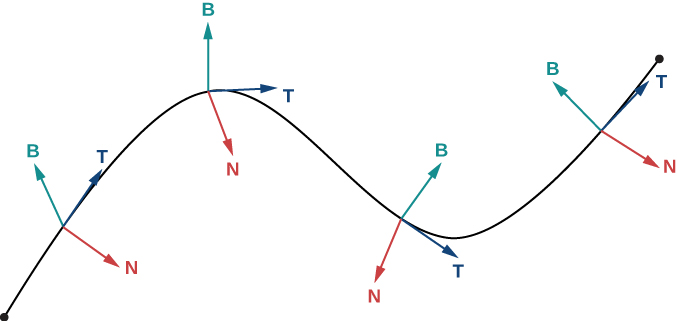
For any smooth curve in three dimensions that is defined by a vector-valued function, we now have formulas for the unit tangent vector \(\vecs T\), the unit normal vector \(\vecs N\), and the binormal vector \(\vecs B\). The unit normal vector and the binormal vector form a plane that is perpendicular to the curve at any point on the curve, called the normal plane. In addition, these three vectors form a frame of reference in three-dimensional space called the Frenet frame of reference (also called the TNB frame) (Figure \(\PageIndex{2}\)). Last, the plane determined by the vectors \(\vecs T\) and \(\vecs N\) forms the osculating plane of \(C\) at any point \(P\) on the curve.
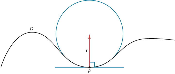
Suppose we form a circle in the osculating plane of \(C\) at point \(P\) on the curve. Assume that the circle has the same curvature as the curve does at point \(P\) and let the circle have radius \(r\). Then, the curvature of the circle is given by \(\frac{1}{r}\). We call \(r\) the radius of curvature of the curve, and it is equal to the reciprocal of the curvature. If this circle lies on the concave side of the curve and is tangent to the curve at point \(P\), then this circle is called the osculating circle of \(C\) at \(P\), as shown in Figure \(\PageIndex{3}\).
For more information on osculating circles, see this demonstration on curvature and torsion, this article on osculating circles, and this discussion of Serret formulas.
To find the equation of an osculating circle in two dimensions, we need find only the center and radius of the circle.
Example \(\PageIndex{5}\): Finding the Equation of an Osculating Circle
Find the equation of the osculating circle of the curve defined by the function \(y=x^3−3x+1\) at \(x=1\).
Solution
Figure \(\PageIndex{4}\) shows the graph of \(y=x^3−3x+1\).
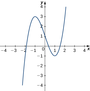
First, let’s calculate the curvature at \(x=1\):
\[κ =\dfrac{|f^{\,\prime\prime}(x)|}{\bigg( 1+[f^{\,\prime}(x)]^2 \bigg) ^{3/2}} = \dfrac{|6x|}{(1+[3x^2−3]^2)^{3/2}}.\]
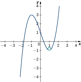
This gives \(κ=6\). Therefore, the radius of the osculating circle is given by \(R=\frac{1}{κ}=\dfrac{1}{6}\). Next, we then calculate the coordinates of the center of the circle. When \(x=1\), the slope of the tangent line is zero. Therefore, the center of the osculating circle is directly above the point on the graph with coordinates \((1,−1)\). The center is located at \((1,−\frac{5}{6})\). The formula for a circle with radius \(r\) and center \((h,k)\) is given by \((x−h)^2+(y−k)^2=r^2\). Therefore, the equation of the osculating circle is \((x−1)^2+(y+\frac{5}{6})^2=\frac{1}{36}\). The graph and its osculating circle appears in the following graph.
Exercise \(\PageIndex{5}\)
Find the equation of the osculating circle of the curve defined by the vector-valued function \(y=2x^2−4x+5\) at \(x=1\).
- Hint
-
Use \(\ref{EqK4}\) to find the curvature of the graph, then draw a graph of the function around \(x=1\) to help visualize the circle in relation to the graph.
- Answer
-
\(κ =\frac{4}{[1+(4x−4)^2]^{3/2}}\)
At the point \(x=1\), the curvature is equal to \(4\). Therefore, the radius of the osculating circle is \(\frac{1}{4}\).
A graph of this function appears next:
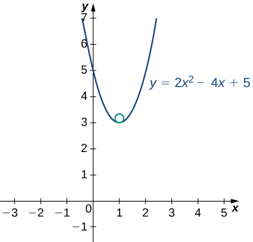
The vertex of this parabola is located at the point \((1,3)\). Furthermore, the center of the osculating circle is directly above the vertex. Therefore, the coordinates of the center are \((1,\frac{13}{4})\). The equation of the osculating circle is
\((x−1)^2+(y−\frac{13}{4})^2=\frac{1}{16}\).
Key Concepts
- The arc-length function for a vector-valued function is calculated using the integral formula \(\displaystyle s(t)=\int_a^b ‖\vecs r^{\,\prime}(t)‖\,dt \). This formula is valid in both two and three dimensions.
- The curvature of a curve at a point in either two or three dimensions is defined to be the curvature of the inscribed circle at that point. The arc-length parameterization is used in the definition of curvature.
- There are several different formulas for curvature. The curvature of a circle is equal to the reciprocal of its radius.
- The principal unit normal vector at \(t\) is defined to be
\[\vecs N(t)=\dfrac{\vecs T^{\,\prime}(t)}{‖\vecs T^{\,\prime}(t)‖}. \nonumber\]
- The binormal vector at \(t\) is defined as \(\vecs B(t)=\vecs T(t)×\vecs N(t)\), where \(\vecs T(t)\) is the unit tangent vector.
- The Frenet frame of reference is formed by the unit tangent vector, the principal unit normal vector, and the binormal vector.
- The osculating circle is tangent to a curve at a point and has the same curvature as the tangent curve at that point.
Key Equations
- Arc length of space curve
\(s= {\displaystyle \int _a^b} \sqrt{[f^{\,\prime}(t)]^2+[g^{\,\prime}(t)]^2+[h^{\,\prime}(t)]^2} \,dt= {\displaystyle \int _a^b} ‖\vecs r^{\,\prime}(t)‖\,dt\) - Arc-length function
\(s(t)={\displaystyle \int _a^t} \sqrt{f^{\,\prime}(u))^2+(g^{\,\prime}(u))^2+(h^{\,\prime}(u))^2} \,du \; or \; s(t)={\displaystyle \int _a^t}‖\vecs r^{\,\prime}(u)‖\,du\) - Curvature
\(κ=\frac{‖\vecs T^{\,\prime}(t)‖}{‖\vecs r^{\,\prime}(t)‖} \; or \; κ=\frac{‖\vecs r^{\,\prime}(t)×\vecs r^{\,\prime\prime}(t)‖}{‖\vecs r^{\,\prime}(t)‖^3} \; or \; κ=\frac{|y^{\,\prime\prime}|}{[1+(y^{\,\prime})^2]^{3/2}}\)
- Principal unit normal vector
\(\vecs N(t)=\frac{\vecs T^{\,\prime}(t)}{‖\vecs T^{\,\prime}(t)‖}\) - Binormal vector
\(\vecs B(t)=\vecs T(t)×\vecs N(t)\)
- arc-length function
- a function \(s(t)\) that describes the arc length of curve \(C\) as a function of \(t\)
- arc-length parameterization
- a reparameterization of a vector-valued function in which the parameter is equal to the arc length
- binormal vector
- a unit vector orthogonal to the unit tangent vector and the unit normal vector
- curvature
- the derivative of the unit tangent vector with respect to the arc-length parameter
- Frenet frame of reference
- (TNB frame) a frame of reference in three-dimensional space formed by the unit tangent vector, the unit normal vector, and the binormal vector
- normal plane
- a plane that is perpendicular to a curve at any point on the curve
- osculating circle
- a circle that is tangent to a curve \(C\) at a point \(P\) and that shares the same curvature
- osculating plane
- the plane determined by the unit tangent and the unit normal vector
- principal unit normal vector
- a vector orthogonal to the unit tangent vector, given by the formula \(\frac{\vecs T^{\,\prime}(t)}{‖\vecs T^{\,\prime}(t)‖}\)
- radius of curvature
- the reciprocal of the curvature
- smooth
- curves where the vector-valued function \(\vecs r(t)\) is differentiable with a non-zero derivative
Contributors
Gilbert Strang (MIT) and Edwin “Jed” Herman (Harvey Mudd) with many contributing authors. This content by OpenStax is licensed with a CC-BY-SA-NC 4.0 license. Download for free at http://cnx.org.