5.1: Derivatives of Exponential Functions.

Exponential functions are often used to describe the growth or decline of biological populations, distribution of enzymes over space, and other biological and chemical relations. The rate of change of exponential functions describes population growth rate, decay of chemical concentration with space, and rates of change of other biological and chemical processes.

The exponential function \(E(t)=2^t\) (where the base is 2 and the exponent is \(t\)) is quite different from the algebraic function, \(P(t)=t^2\) (where the base is tt and the exponent is 2). \(P(t)=t^2\) is well defined for all numbers tt in terms of multiplication, \(P(t)=t \times t\). However, in elementary courses \(2^t\) is defined only for \(t\) a rational number. For the irrational number \(\sqrt{2}=1.4142135 \cdots\), for example, \(2^{\sqrt{2}}\) is the number to which the sequence \(2^{1.4}, ~ 2^{1.41}, ~ 2^{1.414}, ~ 2^{1.4142}, \cdots\) approaches. We will not formalize this idea, but will assume that \(2^t\) is meaningful for all numbers \(t\).

Shown in Table 5.1 are computations and a graph directed to finding the rate of growth of \(E(t)=2^t\) at \(t=2\). We wish to find a number \(m_2\) so that

\[\lim _{b \rightarrow 2}=\frac{2^{b}-2^{2}}{b-2}=m_{2}\]

Table 5.1: Table and Graph of \(E(t) = 2^t\) near \(t = 2\).

\(b\)	\(\frac{2^{b}-2^{2}}{b-2}\)
1.8	2.5890
1.95	2.72509
1.99
1.995	2.76778
1.9999	2.7724926
\(\downarrow\)	\(\downarrow\)
2	\(E ^{\prime} (2)\)
\(\uparrow\)	\(\uparrow\)
2.0001	2.7726848
2.005	2.77740
2.01
2.05	2.82119
2.2	2.9730

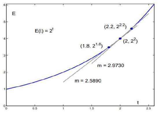
Explore 5.1.1 Compute the two entries corresponding to \(b = 1.99\) and \(b = 2.01\) that are omitted from Table 5.1.

Within the accuracy of Table 5.1, you may conclude that \(m_2\) should be between 2.7724926 and 2.7726848. The average of 2.7724926 and 2.7726848 is a good estimate of \(m_2\).

\[\frac{m_{[2,1.9999]}+m_{[2,2.0001]}}{2}=\frac{2.7724926+2.7726848}{2}=2.7725887\]

We will find in Example ?? that correct to 11 digits, the rate of growth of \(E(t)\) at \(t = 2\) is 2.7725887222. As approximations to \(E ^{\prime} (2)\), 2.7724926 and 2.7726848 are correct to only five digits, but their average, 2.7725887, is correct to all eight digits shown. Such improvement in accuracy by averaging left and right difference quotients (defined next) is common.

For \(P\) a function, the fraction,

\[\frac{P(b)-P(a)}{b-a},\]

is called a difference quotient for \(P\). If \(h > 0\) then the backward, and centered, and forward difference quotients at \(a\) are

\[\begin{array}{ccc}
\text { Backward } & \text { Centered } & \text { Forward } \\
\frac{P(a)-P(a-h)}{h} & \frac{P(a+h)-P(a-h)}{2 h} & \frac{P(a+h)-P(a)}{h}
\end{array}\]

Assuming the interval size \(h\) is the same in all three, the centered difference quotient is the average of the backward and forward difference quotients.

\[\begin{array}\
\frac{\frac{P(a-h)-P(a)}{-h}+\frac{P(a+h)-P(a)}{h}}{2} &=\frac{\frac{-P(a-h)+P(a)}{h}+\frac{P(a+h)-P(a)}{h}}{2} \\
&=\frac{-P(a-h)+P(a)+P(a+h)-P(a)}{2 h} \\
&=\frac{P(a+h)-P(a-h)}{2 h}
\end{array} \label{5.1}\]

The graphs in Figure \ref{5.1} suggest, and it is generally true, that the centered difference quotient is a better approximation to the slope of the tangent to \(P\) at \((a, P(a))\) than is either the forward or backward difference quotients. Formal analysis of the errors in the two approximations appears in Example 12.7.3, Equations 12.22 and 12.23. We will use the centered difference quotient to approximate \(E ^{\prime} (a)\) throughout this chapter.

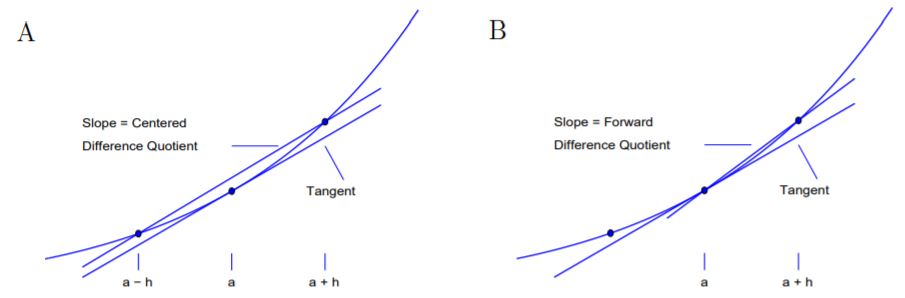
Figure \(\PageIndex{1}\): The centered difference quotient shown in A is closer to the slope of the tangent at \((a, f(a))\) than is the forward difference quotient shown in B.

Using the centered difference approximation, we approximate \(E ^{\prime} (t)\) for \(E(t) = 2^t\) and five different value of \(t\), -1, 0, 1, 2, and 3.

\[\begin{array}{rlrlr} 
& \text { Centered diff quot } & E^{\prime}(t) \doteq & E^{\prime}(t) & E(t) \\
E^{\prime}(-1) & \doteq \frac{2^{-1+0.0001}-2^{-1-0.0001}}{0.0002}&=0.34657359 & 0.35 & \frac{1}{2} \\
E^{\prime}(0) & \doteq \frac{2^{0+0.0001}-2^{0-0.0001}}{0.0002}&=0.69314718 & 0.69 & 1 \\
E^{\prime}(1) & \doteq \frac{2^{1+0.0001}-2^{1-0.0001}}{0.0002} & =1.3862944 & 1.39 & 2 \\
E^{\prime}(2) & \doteq \frac{2^{2+0.0001}-2^{2-0.0001}}{0.0002} & =2.7725887 & 2.77 & 4 \\
E^{\prime}(3) & \doteq \frac{2^{3+0.0001}-2^{3-0.0001}}{0.0002} & =5.5451774 & 5.55 & 8
\end{array}\]

Explore 5.1.2 Do This. An elegant pattern emerges from the previous computations. To help you find it the last two columns contain truncated approximations to \(E ^{\prime} (t)\) and the values of \(E(t)\). Spend at least two minutes looking for the pattern (or less if you find it).

The pattern we hope you see is that

\[E^{\prime}(t) \doteq E^{\prime}(0) E(t)\]

We will soon show that for \(E(t) = 2^t\), \(E ^{\prime} (t) = E ^{\prime} (0) E(t)\), exactly. Meanwhile we observe that \(E ^{\prime} (0) \doteq 0.69314718\) and

\[\begin{aligned}
E^{\prime}(0) E(-1) \doteq 0.69314718 \frac{1}{2}=0.34657359 &\doteq E^{\prime}(-1),\\
E^{\prime}(0) E(1) \doteq 0.69314718 \times 2=1.38629436 &\doteq E^{\prime}(1),\\
E^{\prime}(0) E(2) \doteq 0.69314718 \times 4=2.77258872 &\doteq E^{\prime}(2), \quad \text{and}\\
E^{\prime}(0) E(3) \doteq 0.69314718 \times 8=5.54517744 &\doteq E^{\prime}(3),\\
\end{aligned}\]

which supports the pattern.

Explore 5.1.3 Let \(E(t) = 3^t\). Use the centered difference quotient to approximate \(E ^{\prime} (t)\) for \(t = -1,~ 0,~ 1,~ 2,~ 3\). Test your numbers to see whether \(E^{\prime}(t) \doteq E^{\prime}(0) E(t)\).

The previous work suggests a general rule:

Theorem \(\PageIndex{1}\)

If \(E(t) = B^t\) where \(B > 0\), then

\[E^{\prime}(t)=E^{\prime}(0) E(t) \label{5.2}\]

Proof

For \(E(t) = B^t , ~ B > 0\),

\[\begin{aligned}
E^{\prime}(t)=\lim _{h \rightarrow 0} \frac{B^{t+h}-B^{t}}{h} &=\lim _{h \rightarrow 0} \frac{B^{t} B^{h}-B^{t}}{h}=\lim _{h \rightarrow 0} \frac{B^{t}\left(B^{h}-1\right)}{h} \\
&=B^{t} \lim _{h \rightarrow 0} \frac{B^{h}-B^{0}}{h}=E(t) E^{\prime}(0)
\end{aligned}\]

End of proof.

The preceding argument follows the pattern of all computations of derivatives using Definition 3.3.3. We write the difference quotient, \(\frac{F(t+h)-F(t)}{h}\), balance \(h\) in the denominator with some term in the numerator, and let \(h \rightarrow 0\). In Chapters 3 and 4 we always could factor an \(h\) from the numerator that algebraically canceled the \(h\) in the denominator. In this case, there is no factor, \(h\), in the numerator, but

\[\text { as } h \rightarrow 0, \quad \frac{B^{h}-B^{0}}{h} \rightarrow E^{\prime}(0)\]

and \(h\) in the denominator is neutralized (even though we do not yet know \(E ^{\prime} (0)).

 

Exercises for Section 5.1 Derivatives of Exponential Functions.

Exercise 5.1.1

1. Compute the centered difference \[\frac{P(a+h)-P(a-h)}{2 h}\], which is an approximation to \(P ^{\prime} (a)\), for \(P(t) = t ^2\) and compare your answer with \(P ^{\prime} (a)\).
2. Compute the centered difference \[\frac{P(a+h)-P(a-h)}{2 h}\] for \(P(t) = 5t ^{2} - 3t + 7\) and compare your answer with \(P ^{\prime} (a)\).

Exercise 5.1.2 Technology Sketch the graphs of \(y = 2^t\) and \(y = 4 + 2.7725887(t - 2)\)

1. Using a window of \(0 \leq x \leq 2.5, ~ 0 \leq y \leq 6\).
2. Using a window of \(1.5 \leq x \leq 2.5, ~ 0 \leq y \leq 6\).
3. Using a window of \(1.8 \leq x \leq 2.2, ~ 3.3 \leq y \leq 4.6\).

Mark the point (2,4) on each graph.

Exercise 5.1.3 Let \(E(t) = 10^t\).

1. Approximate \(E ^{\prime} (0)\) using the centered difference quotient on [-0.0001, 0.0001].
2. Use your value for \(E ^{\prime} (0)\) and \(E ^{\prime} (t) = E ^{\prime} (0) E(t)\) to approximate \(E ^{\prime} (-1), ~ E ^{\prime} (1)\), and \(E ^{\prime} (2)\).
3. Sketch the graphs of \(E(t)\) and \(E ^{\prime} (t)\).
4. Repeat a., b., and c. for \(E(t) = 8^t\).

Exercise 5.1.4 Let \(E(t) = (\frac{1}{2})^{t}\).

1. Approximate \(E ^{\prime} (0)\) using the centered difference quotient on [-0.0001, 0.0001].
2. Use your value for \(E ^{\prime} (0)\) and \(E ^{\prime} (t) = E ^{\prime} (0) E(t)\) to approximate \(E ^{\prime} (-1), ~ E ^{\prime} (1)\), and \(E ^{\prime} (2)\).
3. Sketch the graphs of \(E(t)\) and \(E ^{\prime} (t)\).

Exercise 5.1.5 Find (approximately) equations of the lines tangent to the graphs of

1. \(y = 1.5 ^t\) at the points (-1, 2/3), (0, 1), and (1, 3/2)
2. \(y = 2^t\) at the point (-1, 1/2), (0, 1), and (1, 2)
3. \(y = 3^t\) at the point (-1, 1/3), (0, 1), and (1, 3)
4. \(y = 5^t\) at the point (-1, 1/5), (0, 1), and (1, 5)

Exercise 5.1.6 Suppose a bacterium Vibrio natriegens is growing in a beaker and cell concentration \(C\) at time \(t\) in minutes is given by

\[C(t)=0.87 \times 1.02^{t} \quad \text { million cells per } \mathrm{ml}\]

1. Approximate \(C(t)\) and \(C ^{\prime} (t)\) for \(t\) = 0, 10, 20, 30, and 40 minutes.
2. Plot a graph of \(C ^{\prime} (t) ~ vs ~ C(t)\) using the five pairs of values you just computed.

Exercise 5.1.7 Suppose penicillin concentration in the serum of a patient \(t\) minutes after a bolus injection of 2 g is given by

\[P(t)=200 \times 0.96^{t} \quad \mu \mathrm{g} / \mathrm{ml}\]

1. Approximate \(P(t)\) and \(P ^{\prime} (t)\) for \(t\) = 0, 5, 10, 15, and 20 minutes.
2. Plot a graph of \(P ^{\prime} (t) ~ vs ~ P(t)\) using the five pairs of values you just computed.