
2.3.E: Exercises
- Page ID
- 219702

\( \newcommand{\vecs}[1]{\overset { \scriptstyle \rightharpoonup} {\mathbf{#1}} } \)
\( \newcommand{\vecd}[1]{\overset{-\!-\!\rightharpoonup}{\vphantom{a}\smash {#1}}} \)
\( \newcommand{\dsum}{\displaystyle\sum\limits} \)
\( \newcommand{\dint}{\displaystyle\int\limits} \)
\( \newcommand{\dlim}{\displaystyle\lim\limits} \)
\( \newcommand{\id}{\mathrm{id}}\) \( \newcommand{\Span}{\mathrm{span}}\)
( \newcommand{\kernel}{\mathrm{null}\,}\) \( \newcommand{\range}{\mathrm{range}\,}\)
\( \newcommand{\RealPart}{\mathrm{Re}}\) \( \newcommand{\ImaginaryPart}{\mathrm{Im}}\)
\( \newcommand{\Argument}{\mathrm{Arg}}\) \( \newcommand{\norm}[1]{\| #1 \|}\)
\( \newcommand{\inner}[2]{\langle #1, #2 \rangle}\)
\( \newcommand{\Span}{\mathrm{span}}\)
\( \newcommand{\id}{\mathrm{id}}\)
\( \newcommand{\Span}{\mathrm{span}}\)
\( \newcommand{\kernel}{\mathrm{null}\,}\)
\( \newcommand{\range}{\mathrm{range}\,}\)
\( \newcommand{\RealPart}{\mathrm{Re}}\)
\( \newcommand{\ImaginaryPart}{\mathrm{Im}}\)
\( \newcommand{\Argument}{\mathrm{Arg}}\)
\( \newcommand{\norm}[1]{\| #1 \|}\)
\( \newcommand{\inner}[2]{\langle #1, #2 \rangle}\)
\( \newcommand{\Span}{\mathrm{span}}\) \( \newcommand{\AA}{\unicode[.8,0]{x212B}}\)
\( \newcommand{\vectorA}[1]{\vec{#1}} % arrow\)
\( \newcommand{\vectorAt}[1]{\vec{\text{#1}}} % arrow\)
\( \newcommand{\vectorB}[1]{\overset { \scriptstyle \rightharpoonup} {\mathbf{#1}} } \)
\( \newcommand{\vectorC}[1]{\textbf{#1}} \)
\( \newcommand{\vectorD}[1]{\overrightarrow{#1}} \)
\( \newcommand{\vectorDt}[1]{\overrightarrow{\text{#1}}} \)
\( \newcommand{\vectE}[1]{\overset{-\!-\!\rightharpoonup}{\vphantom{a}\smash{\mathbf {#1}}}} \)
\( \newcommand{\vecs}[1]{\overset { \scriptstyle \rightharpoonup} {\mathbf{#1}} } \)
\(\newcommand{\longvect}{\overrightarrow}\)
\( \newcommand{\vecd}[1]{\overset{-\!-\!\rightharpoonup}{\vphantom{a}\smash {#1}}} \)
\(\newcommand{\avec}{\mathbf a}\) \(\newcommand{\bvec}{\mathbf b}\) \(\newcommand{\cvec}{\mathbf c}\) \(\newcommand{\dvec}{\mathbf d}\) \(\newcommand{\dtil}{\widetilde{\mathbf d}}\) \(\newcommand{\evec}{\mathbf e}\) \(\newcommand{\fvec}{\mathbf f}\) \(\newcommand{\nvec}{\mathbf n}\) \(\newcommand{\pvec}{\mathbf p}\) \(\newcommand{\qvec}{\mathbf q}\) \(\newcommand{\svec}{\mathbf s}\) \(\newcommand{\tvec}{\mathbf t}\) \(\newcommand{\uvec}{\mathbf u}\) \(\newcommand{\vvec}{\mathbf v}\) \(\newcommand{\wvec}{\mathbf w}\) \(\newcommand{\xvec}{\mathbf x}\) \(\newcommand{\yvec}{\mathbf y}\) \(\newcommand{\zvec}{\mathbf z}\) \(\newcommand{\rvec}{\mathbf r}\) \(\newcommand{\mvec}{\mathbf m}\) \(\newcommand{\zerovec}{\mathbf 0}\) \(\newcommand{\onevec}{\mathbf 1}\) \(\newcommand{\real}{\mathbb R}\) \(\newcommand{\twovec}[2]{\left[\begin{array}{r}#1 \\ #2 \end{array}\right]}\) \(\newcommand{\ctwovec}[2]{\left[\begin{array}{c}#1 \\ #2 \end{array}\right]}\) \(\newcommand{\threevec}[3]{\left[\begin{array}{r}#1 \\ #2 \\ #3 \end{array}\right]}\) \(\newcommand{\cthreevec}[3]{\left[\begin{array}{c}#1 \\ #2 \\ #3 \end{array}\right]}\) \(\newcommand{\fourvec}[4]{\left[\begin{array}{r}#1 \\ #2 \\ #3 \\ #4 \end{array}\right]}\) \(\newcommand{\cfourvec}[4]{\left[\begin{array}{c}#1 \\ #2 \\ #3 \\ #4 \end{array}\right]}\) \(\newcommand{\fivevec}[5]{\left[\begin{array}{r}#1 \\ #2 \\ #3 \\ #4 \\ #5 \\ \end{array}\right]}\) \(\newcommand{\cfivevec}[5]{\left[\begin{array}{c}#1 \\ #2 \\ #3 \\ #4 \\ #5 \\ \end{array}\right]}\) \(\newcommand{\mattwo}[4]{\left[\begin{array}{rr}#1 \amp #2 \\ #3 \amp #4 \\ \end{array}\right]}\) \(\newcommand{\laspan}[1]{\text{Span}\{#1\}}\) \(\newcommand{\bcal}{\cal B}\) \(\newcommand{\ccal}{\cal C}\) \(\newcommand{\scal}{\cal S}\) \(\newcommand{\wcal}{\cal W}\) \(\newcommand{\ecal}{\cal E}\) \(\newcommand{\coords}[2]{\left\{#1\right\}_{#2}}\) \(\newcommand{\gray}[1]{\color{gray}{#1}}\) \(\newcommand{\lgray}[1]{\color{lightgray}{#1}}\) \(\newcommand{\rank}{\operatorname{rank}}\) \(\newcommand{\row}{\text{Row}}\) \(\newcommand{\col}{\text{Col}}\) \(\renewcommand{\row}{\text{Row}}\) \(\newcommand{\nul}{\text{Nul}}\) \(\newcommand{\var}{\text{Var}}\) \(\newcommand{\corr}{\text{corr}}\) \(\newcommand{\len}[1]{\left|#1\right|}\) \(\newcommand{\bbar}{\overline{\bvec}}\) \(\newcommand{\bhat}{\widehat{\bvec}}\) \(\newcommand{\bperp}{\bvec^\perp}\) \(\newcommand{\xhat}{\widehat{\xvec}}\) \(\newcommand{\vhat}{\widehat{\vvec}}\) \(\newcommand{\uhat}{\widehat{\uvec}}\) \(\newcommand{\what}{\widehat{\wvec}}\) \(\newcommand{\Sighat}{\widehat{\Sigma}}\) \(\newcommand{\lt}{<}\) \(\newcommand{\gt}{>}\) \(\newcommand{\amp}{&}\) \(\definecolor{fillinmathshade}{gray}{0.9}\)2.3 Exercises
What is the slope of the line through (3,9) and \((x, y)\) for \(y = x^2\) and \(x = 2.97\)? \(x = 3.001\)? \(x = 3+h\)? What happens to this last slope when \(h\) is very small (close to 0)? Sketch the graph of \(y = x^2\) for \(x\) near 3.
What is the slope of the line through (–2,4) and \((x, y)\) for \(y = x^2\) and \(x = –1.98\)? \(x = –2.03\)? \(x = –2+h\)? What happens to this last slope when \(h \) is very small (close to 0)? Sketch the graph of \(y = x^2\) for \(x\) near –2.
What is the slope of the line through (2,4) and \((x, y)\) for \(y = x^2 + x – 2\) and \(x = 1.99\)?
\(x = 2.004\)? \(x = 2+h\)? What happens to this last slope when \(h\) is very small? Sketch the graph of \(y = x^2 + x – 2\) for \(x\) near 2.
What is the slope of the line through (–1,–2) and \((x, y)\) for \(y = x^2 +x – 2\) and \(x = –.98\)?
\(x = –1.03\)? \(x = –1+h\)? What happens to this last slope when \(h\) is very small? Sketch the graph of \(y = x^2 + x – 2\) for \(x\) near –1.
The graph to the right shows the temperature during a day in Ames.
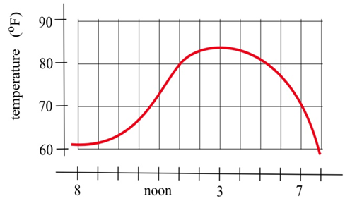
(a) What was the average change in temperature from 9 am to 1 pm?
(b) Estimate how fast the temperature was rising at 10 am and at 7 pm?
The graph shows the distance of a car from a measuring position located on the edge of a straight road.
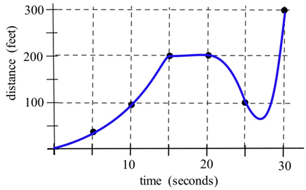
(a) What was the average velocity of the car from \(t = 0\) to \(t = 30\) seconds?
(b) What was the average velocity of the car from \(t = 10\) to \(t = 30\) seconds?
(c) About how fast was the car traveling at \(t = 10\) seconds? at \(t = 20\) s? at \(t = 30\) s?
(d) What does the horizontal part of the graph between \(t = 15\) and \(t = 20\) seconds mean?
(e) What does the negative velocity at \(t = 25\) represent?
The graph shows the distance of a car from a measuring position located on the edge of a straight road.
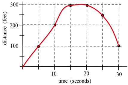
(a) What was the average velocity of the car from \(t = 0\) to \(t = 20\) seconds?
(b) What was the average velocity from \(t = 10\) to \(t = 30\) seconds?
(c) About how fast was the car traveling at \(t = 10\) seconds? at \(t = 20\) s? at \(t = 30\) s?
The graph shows the composite developmental skill level of chessmasters at different ages as determined by their performance against other chessmasters. (From "Rating Systems for Human Abilities", by W.H. Batchelder and R.S. Simpson, 1988. UMAP Module 698.)
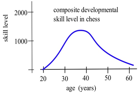
(a) At what age is the "typical" chessmaster playing the best chess?
(b) At approximately what age is the chessmaster's skill level increasing most rapidly?
(c) Describe the development of the "typical" chessmaster's skill in words.
(d) Sketch graphs which you think would reasonably describe the performance levels versus age for an athlete, a classical pianist, a rock singer, a mathematician, and a professional in your major field.
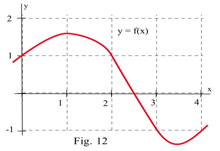
Use the function in the graph to fill in the table and then graph \(m(x)\).
| \(x\) | \(y = f(x)\) | \(m(x) = \) the estimated slope of the tangent line to \(y=f(x)\) at the point \((x,y)\) |
| 0 | ||
| 0.5 | ||
| 1.0 | ||
| 1.5 | ||
| 2.0 | ||
| 2.5 | ||
| 3.0 | ||
| 3.5 | ||
| 4.0 |
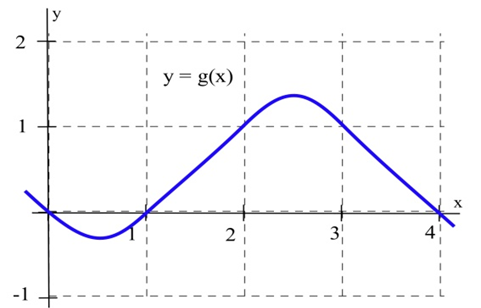
Use the function in the graph to fill in the table and then graph \(m(x)\).
| \(x\) | \(y = g(x)\) | \(m(x) = \) the estimated slope of the tangent line to \(y=g(x)\) at the point \((x,y)\) |
| 0 | ||
| 0.5 | ||
| 1.0 | ||
| 1.5 | ||
| 2.0 | ||
| 2.5 | ||
| 3.0 | ||
| 3.5 | ||
| 4.0 |
(a) At what values of \(x\) does the graph of \(f\) in the graph have a horizontal tangent line?
(b) At what value(s) of \(x\) is the value of \(f\) the largest? smallest?
(c) Sketch the graph of \(m(x)\) = the slope of the line tangent to the graph of \(f\) at the point \((x,y)\)
(a) At what values of \(x\) does the graph of \(g\) have a horizontal tangent line?
(b) At what value(s) of \(x\) is the value of \(g\) the largest? smallest?
(c) Sketch the graph of \(m(x) =\) the slope of the line tangent to the graph of \(g\) at the point \((x,y)\).
Match the situation descriptions with the corresponding time–velocity graph.
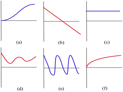
(a) A car quickly leaving from a stop sign.
(b) A car sedately leaving from a stop sign.
(c) A student bouncing on a trampoline.
(d) A ball thrown straight up.
(e) A student confidently striding across campus to take a calculus test.
(f) An unprepared student walking across campus to take a calculus test.
For each function \(f(x)\) in problems 14 – 19, perform steps (a) – (d):
(a) calculate \(m_{\sec} = \frac{f(x+h)-f(x)}{h}\) and simplify
(b) determine \(m_{\tan} = \lim_{h \to 0} m_{\sec}\)
(c) evaluate \(m_{\tan} \) at \(x = 2\),
(d) find the equation of the line tangent to the graph of \(f\) at \((2, f(2) )\)
| 14. \(f(x) = 3x – 7\) | 15. \(f(x) = 2 – 7x\) | 16. \(f(x) = ax + b\) where \(a\) and \(b\) are constants |
| 17. \(f(x) = x^2 + 3x\) | 18. \(f(x) = 8 – 3x^2\) | 19. \(f(x) = ax^2 + bx + c\) where \(a\), \(b\) and \(c\) are constants |
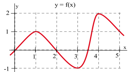
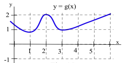
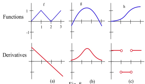
Match the graphs of the three functions below with the graphs of their derivatives.
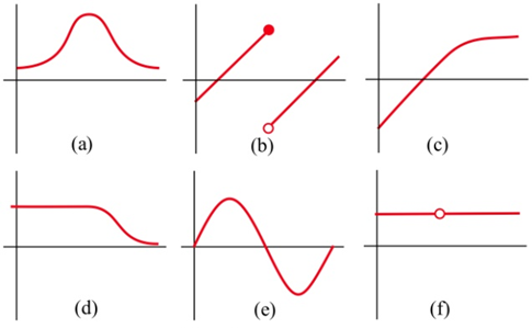
Below are six graphs, three of which are derivatives of the other three. Match the functions with their derivatives.
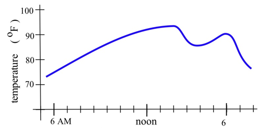
The graph below shows the temperature during a summer day in Chicago. Sketch the graph of the rate at which the temperature is changing. (This is just the graph of the slopes of the lines which are tangent to the temperature graph.)
Fill in the table with the appropriate units for \(f '(x)\).
|
units for \(x\) |
units for \(f(x)\) |
units for \(f '(x)\) |
|
hours |
miles |
|
|
people |
automobiles |
|
|
dollars |
pancakes |
|
|
days |
trout |
|
|
seconds |
miles per second |
|
|
seconds |
gallons |
|
|
study hours |
test points |
If \(C(x)\) is the total cost, in millions, of producing \(x\) thousand items, interpret \(C'(4) = 2\).
Suppose \(P(t)\) is the number of individuals infected by a disease \(t\) days after it was first detected. Interpret \(P'(50) = -200\).