6.1: Introduction to Differential Equations

Last updated
Save as PDF

Page ID: 212055

$ \newcommand{\vecs}[1]{\overset { \scriptstyle \rightharpoonup} {\mathbf{#1}} } $

$ \newcommand{\vecd}[1]{\overset{-\!-\!\rightharpoonup}{\vphantom{a}\smash {#1}}} $

$ \newcommand{\dsum}{\displaystyle\sum\limits} $

$ \newcommand{\dint}{\displaystyle\int\limits} $

$ \newcommand{\dlim}{\displaystyle\lim\limits} $

$ \newcommand{\id}{\mathrm{id}}$ $ \newcommand{\Span}{\mathrm{span}}$

( \newcommand{\kernel}{\mathrm{null}\,}\) $ \newcommand{\range}{\mathrm{range}\,}$

$ \newcommand{\RealPart}{\mathrm{Re}}$ $ \newcommand{\ImaginaryPart}{\mathrm{Im}}$

$ \newcommand{\Argument}{\mathrm{Arg}}$ $ \newcommand{\norm}[1]{\| #1 \|}$

$ \newcommand{\inner}[2]{\langle #1, #2 \rangle}$

$ \newcommand{\Span}{\mathrm{span}}$

$ \newcommand{\id}{\mathrm{id}}$

$ \newcommand{\Span}{\mathrm{span}}$

$ \newcommand{\kernel}{\mathrm{null}\,}$

$ \newcommand{\range}{\mathrm{range}\,}$

$ \newcommand{\RealPart}{\mathrm{Re}}$

$ \newcommand{\ImaginaryPart}{\mathrm{Im}}$

$ \newcommand{\Argument}{\mathrm{Arg}}$

$ \newcommand{\norm}[1]{\| #1 \|}$

$ \newcommand{\inner}[2]{\langle #1, #2 \rangle}$

$ \newcommand{\Span}{\mathrm{span}}$ $ \newcommand{\AA}{\unicode[.8,0]{x212B}}$

$ \newcommand{\vectorA}[1]{\vec{#1}} % arrow$

$ \newcommand{\vectorAt}[1]{\vec{\text{#1}}} % arrow$

$ \newcommand{\vectorB}[1]{\overset { \scriptstyle \rightharpoonup} {\mathbf{#1}} } $

$ \newcommand{\vectorC}[1]{\textbf{#1}} $

$ \newcommand{\vectorD}[1]{\overrightarrow{#1}} $

$ \newcommand{\vectorDt}[1]{\overrightarrow{\text{#1}}} $

$ \newcommand{\vectE}[1]{\overset{-\!-\!\rightharpoonup}{\vphantom{a}\smash{\mathbf {#1}}}} $

$ \newcommand{\vecs}[1]{\overset { \scriptstyle \rightharpoonup} {\mathbf{#1}} } $

$\newcommand{\longvect}{\overrightarrow}$

$ \newcommand{\vecd}[1]{\overset{-\!-\!\rightharpoonup}{\vphantom{a}\smash {#1}}} $

$\newcommand{\avec}{\mathbf a}$ $\newcommand{\bvec}{\mathbf b}$ $\newcommand{\cvec}{\mathbf c}$ $\newcommand{\dvec}{\mathbf d}$ $\newcommand{\dtil}{\widetilde{\mathbf d}}$ $\newcommand{\evec}{\mathbf e}$ $\newcommand{\fvec}{\mathbf f}$ $\newcommand{\nvec}{\mathbf n}$ $\newcommand{\pvec}{\mathbf p}$ $\newcommand{\qvec}{\mathbf q}$ $\newcommand{\svec}{\mathbf s}$ $\newcommand{\tvec}{\mathbf t}$ $\newcommand{\uvec}{\mathbf u}$ $\newcommand{\vvec}{\mathbf v}$ $\newcommand{\wvec}{\mathbf w}$ $\newcommand{\xvec}{\mathbf x}$ $\newcommand{\yvec}{\mathbf y}$ $\newcommand{\zvec}{\mathbf z}$ $\newcommand{\rvec}{\mathbf r}$ $\newcommand{\mvec}{\mathbf m}$ $\newcommand{\zerovec}{\mathbf 0}$ $\newcommand{\onevec}{\mathbf 1}$ $\newcommand{\real}{\mathbb R}$ $\newcommand{\twovec}[2]{\left[\begin{array}{r}#1 \\ #2 \end{array}\right]}$ $\newcommand{\ctwovec}[2]{\left[\begin{array}{c}#1 \\ #2 \end{array}\right]}$ $\newcommand{\threevec}[3]{\left[\begin{array}{r}#1 \\ #2 \\ #3 \end{array}\right]}$ $\newcommand{\cthreevec}[3]{\left[\begin{array}{c}#1 \\ #2 \\ #3 \end{array}\right]}$ $\newcommand{\fourvec}[4]{\left[\begin{array}{r}#1 \\ #2 \\ #3 \\ #4 \end{array}\right]}$ $\newcommand{\cfourvec}[4]{\left[\begin{array}{c}#1 \\ #2 \\ #3 \\ #4 \end{array}\right]}$ $\newcommand{\fivevec}[5]{\left[\begin{array}{r}#1 \\ #2 \\ #3 \\ #4 \\ #5 \\ \end{array}\right]}$ $\newcommand{\cfivevec}[5]{\left[\begin{array}{c}#1 \\ #2 \\ #3 \\ #4 \\ #5 \\ \end{array}\right]}$ $\newcommand{\mattwo}[4]{\left[\begin{array}{rr}#1 \amp #2 \\ #3 \amp #4 \\ \end{array}\right]}$ $\newcommand{\laspan}[1]{\text{Span}\{#1\}}$ $\newcommand{\bcal}{\cal B}$ $\newcommand{\ccal}{\cal C}$ $\newcommand{\scal}{\cal S}$ $\newcommand{\wcal}{\cal W}$ $\newcommand{\ecal}{\cal E}$ $\newcommand{\coords}[2]{\left\{#1\right\}_{#2}}$ $\newcommand{\gray}[1]{\color{gray}{#1}}$ $\newcommand{\lgray}[1]{\color{lightgray}{#1}}$ $\newcommand{\rank}{\operatorname{rank}}$ $\newcommand{\row}{\text{Row}}$ $\newcommand{\col}{\text{Col}}$ $\renewcommand{\row}{\text{Row}}$ $\newcommand{\nul}{\text{Nul}}$ $\newcommand{\var}{\text{Var}}$ $\newcommand{\corr}{\text{corr}}$ $\newcommand{\len}[1]{\left|#1\right|}$ $\newcommand{\bbar}{\overline{\bvec}}$ $\newcommand{\bhat}{\widehat{\bvec}}$ $\newcommand{\bperp}{\bvec^\perp}$ $\newcommand{\xhat}{\widehat{\xvec}}$ $\newcommand{\vhat}{\widehat{\vvec}}$ $\newcommand{\uhat}{\widehat{\uvec}}$ $\newcommand{\what}{\widehat{\wvec}}$ $\newcommand{\Sighat}{\widehat{\Sigma}}$ $\newcommand{\lt}{<}$ $\newcommand{\gt}{>}$ $\newcommand{\amp}{&}$ $\definecolor{fillinmathshade}{gray}{0.9}$

Algebraic equations involve constants and variables, and solutions of algebraic equations typically involve numbers. For example, $x = 3$ and $x = -2$ are solutions of the algebraic equation $\displaystyle x^2 = x + 6$. Differential equations contain derivatives (or differentials) of functions and solutions of differential equations are functions. The differential equation $y' = 3x^2$ has infinitely many solutions, and two of those solutions are the functions $y = x^3 + 2$ and $y = x^3 - 4$:

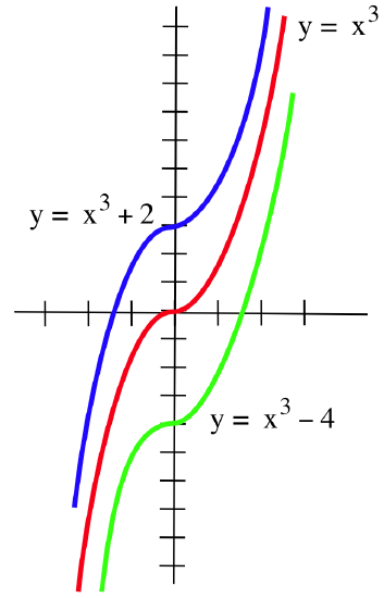
$A red graph of y = x cubed, a blue graph of y = x cubed + 2, and a green graph of y = x cubed - 4.$

You have already solved lots of differential equations: every time you found an antiderivative of a function $f(x)$, you solved the differential equation $y' = f(x)$ to get a solution $y$. You have also used differential equations in applications. Areas, volumes, work and motion problems all involved integration and finding antiderivatives, so they all involved solving a differential equation. The differential equation $y' = f(x)$, however, is just the beginning. Other applications generate differential equations that may involve higher-order derivatives of $y$ (such as $y''$) and functions of $y$ as well as $x$.

Checking Solutions of Differential Equations

Whether a differential equation is easy or difficult to solve, it is important to be able to check that a possible solution actually satisfies the differential equation. A possible solution of an algebraic equation can be checked by putting the solution into the equation to see if it results in true statement: $x = 3$ is a solution of $5x + 1 = 16$ because $5(3) + 1 = 16$ is true; $x = 4$ is not a solution, because $5(4) + 1 \neq 16$.

Similarly, a solution of a differential equation can be checked by substituting the function (and its appropriate derivatives) into the original equation to see if the result is true: $y = x^2$ is a solution of $xy' = 2y$ because $y = x^2 \Rightarrow y' = 2x$ and $\displaystyle x\cdot 2x = 2\cdot x^2$ is a true statement for all values of $x$.

Example $\PageIndex{1}$

Check that:

$y = x^2 + 5$ is a solution of $y'' + y = x^2 + 7$ and
$\displaystyle y = x + \frac{5}{x}$ is a solution of $\displaystyle y' + \frac{y}{x} = 2$.

Solution

$y = x^2 + 5 \Rightarrow y' = 2x \Rightarrow y'' = 2$. Substituting these functions for $y$ and $y''$ into the left side of the differential equation $y'' + y = x^2 + 7$ yields:\[y'' + y = (2) + (x^2 + 5) = x^2 + 7\]so $y = x^2 + 5$ is a solution of the differential equation.
$\displaystyle y = x + \frac{5}{x} \Rightarrow y' = 1 - \frac{5}{x^2}$. Substituting these functions for $y$ and $y'$ into the left side of the differential equation $\displaystyle y' + \frac{y}{x} = 2$, we have:\[y' + \frac{y}{x} = \left[1 - \frac{5}{x^2}\right] + \frac{1}{x}\left[x + \frac{5}{x}\right] = 1 - \frac{5}{x^2} + 1 + \frac{5}{x^2} = 2\]which matches the right side of the original differential equation.

Practice $\PageIndex{1}$

Check that:

$y = 2x + 6$ is a solution of $y - 3y' = 2x$ and
$y = e^{3x}$, $y = 5e^{3x}$ and $y = Ae^{3x}$ (where $A$ is any constant) are all solutions of $y'' - 2y' - 3y = 0$.

Answer

$y = 2x + 6 \Rightarrow y' = 2$; $y - 3y' = (2x+6) - 3(2) = 2x$ (OK)
$y = e^{3x} \Rightarrow y' = 3e^{3x} \Rightarrow y'' = 9e^{3x}$ so:\[y'' - 2y' - 3y = 9e^{3x} - 2(3e^{3x}) - 3(e^{3x}) = 0 \quad \mbox{(OK)}\]\)y = 5e^{3x} \Rightarrow y' = 15e^{3x} \Rightarrow y'' = 45e^{3x}\) so:\[y'' - 2y' - 3y = 45e^{3x} - 2(15e^{3x}) - 3(5e^{3x}) = 0 \quad \mbox{(OK)}\]\)y = Ae^{3x} \Rightarrow y' = 3Ae^{3x} \Rightarrow y'' = 9Ae^{3x}\) so:\[y'' - 2y' - 3y = 9Ae^{3x} - 2(3Ae^{3x}) - 3(Ae^{3x}) = 0 \quad \mbox{(OK)}\]

A solution of a differential equation with the initial condition $y(x_0) = y_0$ is a function that satisfies the differential equation as well as the initial condition. To check the solution of an initial value problem (or IVP), we must check that a solution function satisfies both the equation and the initial condition.

Example $\PageIndex{2}$

Which of the given functions is a solution of the initial value problem $y' = 3y$, $y(0) = 5$?

$y = e^{3x}$
$y = 5e^{3x}$
$y = -2e^{3x}$

Solution

All three functions satisfy the differential equation, but only one of them satisfies the initial condition that $y(0) = 5$. If $y = e^{3x}$, then $y(0) = e^{3(0) }= 1 \neq 5$ so $y = e^{3x}$ does not satisfy the initial condition:

$A red graph of y = e^(3x), a blue graph of y = 5 e^(3x), and a green graph of y = -2 e^(3x).$

If $y = 5e^{3x}$, then $y(0) = 5e^{3(0)} = 5$ so $y = 5e^{3x}$ does satisfy the initial condition. If $y = -2e^{3x}$, then $y(0) = -2e^{3(0)} = -2 \neq 5$ so $y = e^{3x}$ does not satisfy the initial condition.

Practice $\PageIndex{2}$

Which function is a solution of the initial value problem $y'' + 9y = 0$, $y(0) = 2$?

$y = \sin(3x)$
$y = 2\sin(3x)$
$y = 2\cos(3x)$

Answer

We want $y'' + 9y = 0$ and \)y(0) = 2\).

$y = \sin(3x) \Rightarrow y' = 3\cos(3x) \Rightarrow y'' = -9\sin(3x)$ so we have $y''+9y = -9\sin(3x) +9\cdot\sin(3x) = 0$ (OK) but checking the initial condition: $y(0) = \sin(0) = 0 \neq 2$.
$y = 2\sin(3x) \Rightarrow y' = 6\cos(3x) \Rightarrow y'' = -18\sin(3x)$ so we have $y''+9y = -18\sin(3x) +9\cdot 2\sin(3x) = 0$ (OK) but checking the initial condition: $y(0) = 2\sin(0) = 0 \neq 2$
$y = 2\cos(3x) \Rightarrow y' = -6\sin(3x) \Rightarrow y'' = -18\cos(3x)$ so $y''+9y = -18\cos(3x) +9\cdot2\cos(3x) = 0$ (OK) and checking the initial condition: $y(0) = 2\cos(0) = 2$ (OK).

Only $y = 2\cos(3x)$ satisfies both the ODE and the initial condition.

Finding the Value of the Constant

Differential equations usually have many solutions, typically a whole “family” of them, with each solution in the family satisfying a different initial condition. To find which solution of a differential equation also satisfies a given initial condition of the form $y(x_0) = y_0$, we replace $x$ and $y$ in an equation describing the solution family with the values $x_0$ and $y_0$, then algebraically solve for the value of an unknown constant.

Example $\PageIndex{3}$

For every value of $C$, the function $y = Cx^2$ is a solution of $xy' = 2y$:

$A red graph of y = 4 x squared, a blue graph of y = x squared, and a green graph of y = 1/2 x squared.$

Find the value of $C$ so that $y(5) = 50$.

Solution

Substituting the initial condition $x = 5$ and $y = 50$ into the solution $y = Cx^2$:\[50 = C(5^2) \ \Rightarrow \ C = \frac{50}{25} = 2\]so the function $y = 2x^2$ satisfies both the differential equation and the initial condition.

Practice $\PageIndex{3}$

For every value of $C$, the function $y = e^{2x} + C$ is a solution of $y' = 2e^{2x}$. Find the value of $C$ so that $y(0) = 7$.

Answer: $y = e^{2x} + C \Rightarrow y' = 2e^{2x}$ (OK) so, plugging in the initial values:\[7 = y(0) = e^{2\cdot 0} + C \Rightarrow 7 = 1 + C \Rightarrow C = 6\)\]so $y = e^{2x} + 6$.

Types of Differential Equations

In Chapter 14, we will begin studying partial derivatives of functions of more than one variable, which can appear in differential equations called partial differential equations (or PDEs). Because of this, we will call differential equations involving ordinary derivatives, such as $\displaystyle \frac{dy}{dx}$, $\displaystyle \frac{dy}{dt}$ or $\displaystyle \frac{d^2y}{dt^2}$, ordinary differential equations (or ODEs).

Problems

In Problems 1–10, check that the function $y$ is a solution of the given differential equation.

$y' + 3y = 6$; $y = e^{-3x} + 2$
$y' - 2y = 8$; $y = e^{2x} - 4$
$y'' - y' + y = x^2$; $y = x^2 + 2x$
$3y'' + y' + y = x^2 - 4x$; $y = x^2 - 6x$
$xy' - 3y = x^2$; $y = 7x^3 - x^2$
$xy'' - y' = 3$; $y = x^2 - 3x + 5$
$y' + y = e^x$; $y =\frac12 e^x + 2e^{-x}$
$y'' + 25y = 0$; $y = \sin(5x) + 2\cos(5x)$
$\displaystyle y' = -\frac{x}{y}$; $y = \sqrt{7 - x^2}$
$y' = x - y$; $y = x - 1 + 2e^{-x}$

In Problems 11–20, check that the function $y$ is a solution of the given initial value problem.

$y' = 6x^2 - 3$, $y(1) = 2$; $y = 2x^3 - 3x + 3$
$y' = 6x + 4$, $y(2) = 3$; $y = 3x^2 + 4x - 17$
$y' = 2\cos(2x)$, $y(0) = 1$; $y = \sin(2x) + 1$
$y' = 1 + 6\sin(2x)$, $y(0) = 2$; $y = x - 3\cos(2x) + 5$
$y' = 5y$, $y(0) = 7$; $y = 7e^{5x}$
$y' = -2y$, $y(0) = 3$; $y = 3e^{-2x}$
$xy' = -y$, $y(1) = -4$; $\displaystyle y = -\frac{4}{x}$
$y\cdot y' = -x$, $y(0) = 3$; $y = \sqrt{9 - x^2}$
$\displaystyle y' = \frac{5}{x}$, $y(e) = 3$; $y = 5\ln(x) - 2$
$y' + y = e^x$, $y(0) = 5$; $y = \frac12 e^x + \frac92 e^{-x}$

In Problems 21–30, find the value of the constant $C$ so a function from the given family of solutions satisfies the given initial value problem.

$y' = 2x$, $y(3) = 7$; $y = x^2 + C$
$y' = 3x^2 - 5$, $y(1) = 2$; $y = x^3 - 5x + C$
$y' = 3y$, $y(0) = 5$; $y = Ce^{3x}$
$y' = -2y$, $y(0) = 3$; $y = Ce^{-2x}$
$y' = 6\cos(3x)$, $y(0) = 4$; $y = 2\sin(3x) + C$
$y' = 3 - 2\sin(2x)$, $y(0) = 1$; $y = 3x + \cos(2x) + C$
$\displaystyle y' = \frac{1}{x}$, $y(e) = 2$; $y = \ln(x) + C$
$\displaystyle y' = \frac{1}{x^2}$, $y(1) = 3$; $y = -\frac{1}{x} + C$
$\displaystyle y' = -\frac{y}{x}$, $y(2) = 10$; $y = -\frac{C}{x}$
$y' = -\frac{x}{y}$, $y(3) = 4$; $y = \sqrt{C - x^2}$

In Problems 31–40, find the find the function $y$ that satisfies the given initial value problem.

$y' = 4x^2 - x$, $y(1) = 7$
$y' = x - e^x$, $y(0) = 3$
$\displaystyle y' = \frac{3}{x}$, $y(1) = 2$
$xy' = 1$, $y(e) = 7$
$y' = 6e^{2x}$, $y(0) = 1$
$y' = 36(3x - 2)^2$, $y(1) = 8$
$y'= x\cdot\sin(x^2)$, $y(0) = 3$
$\displaystyle y' = \frac{6}{x^2}$, $y(1) = 2$
$xy' = 6x^3 - 10x^2$, $y(2) = 5$
$x^2 y' = 6x^3 - 1$, $y(1) = 10$
Show that if $y = f(x)$ and $y = g(x)$ are both solutions to $y' + 5y = 0$, then $y = 3\cdot f(x)$, $y = 7\cdot g(x)$, $y = f(x) + g(x)$ and $y = A\cdot f(x) + B\cdot g(x)$ are solutions for any constants $A$ and $B$.
Show that if $f(x)$ and $g(x)$ are both solutions to $y'' + 2y' - 3y = 0$, then so are $y = 3\cdot f(x)$, $y = 7\cdot g(x)$, $y = f(x) + g(x)$ and $y = A\cdot f(x) + B\cdot g(x)$ for any constants $A$ and $B$.
Show that $y = \sin(x) + x$ and $y = \cos(x) + x$ are both solutions of $y'' + y = x$. Are $y = 3\left[\sin(x) + x\right]$ and $y = \left[\sin(x) + x\right] + \left[\cos(x) + x\right]$ solutions of $y'' + y = x$?
Show that $y = e^{3x} - 2$ and $y = 5e^{3x} - 2$ are both solutions of $y' - 3y = 6$. Are $y = 7\left[e^{3x} - 2\right]$ and $y = \left[e^{3x} - 2\right] + \left[5e^{3x} - 2\right]$ also solutions?
The ODE $\displaystyle \frac{dy}{dt} = A - By$ (where $A$ and $B$ are positive constants) describes the concentration $y$ of glucose in a person's blood at time $t$. Check that $\displaystyle y = \frac{A}{B} - C\cdot e^{-Bt}$ is a solution of the ODE for any value of the constant $C$.
The ODE $\displaystyle \frac{dy}{dt} = Ay$ (where $A$ is a positive constant) is used to model “exponential'' growth and decay. Check that $\displaystyle y = C\cdot e^{At}$ is a solution of the differential equation for any value of the constant $C$.
The ODE $\displaystyle L\cdot \frac{dI}{dt} + RI = E$ (where $L$, $R$ and $E$ are positive constants) describes the current $I(t)$ in an electrical circuit. Show that $\displaystyle I = \frac{E}{R}\left(1 - e^{-\frac{Rt}{L}}\right)$ is a solution of the ODE.
The ODE $m\cdot y'' + C\cdot y = 0$ (where $C$ is a positive constant) describes the position $y$ of an object hung from a spring as it moves up and down. Show that $y = A\cdot\sin(\omega t) + B\cdot\cos(\omega t)$ with $\displaystyle \omega = \sqrt{\frac{C}{m}}$ is a solution of the ODE for all values of the constants $A$ and $B$.

Search

Text Color

Text Size

Margin Size

Font Type

Example \(\PageIndex{1}\)

Solution

Practice \(\PageIndex{1}\)

Example \(\PageIndex{2}\)

Solution

Practice \(\PageIndex{2}\)

Example \(\PageIndex{3}\)

Solution

Practice \(\PageIndex{3}\)