0.1: A Preview of Calculus

Last updated
Save as PDF

Page ID: 209795

$ \newcommand{\vecs}[1]{\overset { \scriptstyle \rightharpoonup} {\mathbf{#1}} } $

$ \newcommand{\vecd}[1]{\overset{-\!-\!\rightharpoonup}{\vphantom{a}\smash {#1}}} $

$ \newcommand{\dsum}{\displaystyle\sum\limits} $

$ \newcommand{\dint}{\displaystyle\int\limits} $

$ \newcommand{\dlim}{\displaystyle\lim\limits} $

$ \newcommand{\id}{\mathrm{id}}$ $ \newcommand{\Span}{\mathrm{span}}$

( \newcommand{\kernel}{\mathrm{null}\,}\) $ \newcommand{\range}{\mathrm{range}\,}$

$ \newcommand{\RealPart}{\mathrm{Re}}$ $ \newcommand{\ImaginaryPart}{\mathrm{Im}}$

$ \newcommand{\Argument}{\mathrm{Arg}}$ $ \newcommand{\norm}[1]{\| #1 \|}$

$ \newcommand{\inner}[2]{\langle #1, #2 \rangle}$

$ \newcommand{\Span}{\mathrm{span}}$

$ \newcommand{\id}{\mathrm{id}}$

$ \newcommand{\Span}{\mathrm{span}}$

$ \newcommand{\kernel}{\mathrm{null}\,}$

$ \newcommand{\range}{\mathrm{range}\,}$

$ \newcommand{\RealPart}{\mathrm{Re}}$

$ \newcommand{\ImaginaryPart}{\mathrm{Im}}$

$ \newcommand{\Argument}{\mathrm{Arg}}$

$ \newcommand{\norm}[1]{\| #1 \|}$

$ \newcommand{\inner}[2]{\langle #1, #2 \rangle}$

$ \newcommand{\Span}{\mathrm{span}}$ $ \newcommand{\AA}{\unicode[.8,0]{x212B}}$

$ \newcommand{\vectorA}[1]{\vec{#1}} % arrow$

$ \newcommand{\vectorAt}[1]{\vec{\text{#1}}} % arrow$

$ \newcommand{\vectorB}[1]{\overset { \scriptstyle \rightharpoonup} {\mathbf{#1}} } $

$ \newcommand{\vectorC}[1]{\textbf{#1}} $

$ \newcommand{\vectorD}[1]{\overrightarrow{#1}} $

$ \newcommand{\vectorDt}[1]{\overrightarrow{\text{#1}}} $

$ \newcommand{\vectE}[1]{\overset{-\!-\!\rightharpoonup}{\vphantom{a}\smash{\mathbf {#1}}}} $

$ \newcommand{\vecs}[1]{\overset { \scriptstyle \rightharpoonup} {\mathbf{#1}} } $

$\newcommand{\longvect}{\overrightarrow}$

$ \newcommand{\vecd}[1]{\overset{-\!-\!\rightharpoonup}{\vphantom{a}\smash {#1}}} $

$\newcommand{\avec}{\mathbf a}$ $\newcommand{\bvec}{\mathbf b}$ $\newcommand{\cvec}{\mathbf c}$ $\newcommand{\dvec}{\mathbf d}$ $\newcommand{\dtil}{\widetilde{\mathbf d}}$ $\newcommand{\evec}{\mathbf e}$ $\newcommand{\fvec}{\mathbf f}$ $\newcommand{\nvec}{\mathbf n}$ $\newcommand{\pvec}{\mathbf p}$ $\newcommand{\qvec}{\mathbf q}$ $\newcommand{\svec}{\mathbf s}$ $\newcommand{\tvec}{\mathbf t}$ $\newcommand{\uvec}{\mathbf u}$ $\newcommand{\vvec}{\mathbf v}$ $\newcommand{\wvec}{\mathbf w}$ $\newcommand{\xvec}{\mathbf x}$ $\newcommand{\yvec}{\mathbf y}$ $\newcommand{\zvec}{\mathbf z}$ $\newcommand{\rvec}{\mathbf r}$ $\newcommand{\mvec}{\mathbf m}$ $\newcommand{\zerovec}{\mathbf 0}$ $\newcommand{\onevec}{\mathbf 1}$ $\newcommand{\real}{\mathbb R}$ $\newcommand{\twovec}[2]{\left[\begin{array}{r}#1 \\ #2 \end{array}\right]}$ $\newcommand{\ctwovec}[2]{\left[\begin{array}{c}#1 \\ #2 \end{array}\right]}$ $\newcommand{\threevec}[3]{\left[\begin{array}{r}#1 \\ #2 \\ #3 \end{array}\right]}$ $\newcommand{\cthreevec}[3]{\left[\begin{array}{c}#1 \\ #2 \\ #3 \end{array}\right]}$ $\newcommand{\fourvec}[4]{\left[\begin{array}{r}#1 \\ #2 \\ #3 \\ #4 \end{array}\right]}$ $\newcommand{\cfourvec}[4]{\left[\begin{array}{c}#1 \\ #2 \\ #3 \\ #4 \end{array}\right]}$ $\newcommand{\fivevec}[5]{\left[\begin{array}{r}#1 \\ #2 \\ #3 \\ #4 \\ #5 \\ \end{array}\right]}$ $\newcommand{\cfivevec}[5]{\left[\begin{array}{c}#1 \\ #2 \\ #3 \\ #4 \\ #5 \\ \end{array}\right]}$ $\newcommand{\mattwo}[4]{\left[\begin{array}{rr}#1 \amp #2 \\ #3 \amp #4 \\ \end{array}\right]}$ $\newcommand{\laspan}[1]{\text{Span}\{#1\}}$ $\newcommand{\bcal}{\cal B}$ $\newcommand{\ccal}{\cal C}$ $\newcommand{\scal}{\cal S}$ $\newcommand{\wcal}{\cal W}$ $\newcommand{\ecal}{\cal E}$ $\newcommand{\coords}[2]{\left\{#1\right\}_{#2}}$ $\newcommand{\gray}[1]{\color{gray}{#1}}$ $\newcommand{\lgray}[1]{\color{lightgray}{#1}}$ $\newcommand{\rank}{\operatorname{rank}}$ $\newcommand{\row}{\text{Row}}$ $\newcommand{\col}{\text{Col}}$ $\renewcommand{\row}{\text{Row}}$ $\newcommand{\nul}{\text{Nul}}$ $\newcommand{\var}{\text{Var}}$ $\newcommand{\corr}{\text{corr}}$ $\newcommand{\len}[1]{\left|#1\right|}$ $\newcommand{\bbar}{\overline{\bvec}}$ $\newcommand{\bhat}{\widehat{\bvec}}$ $\newcommand{\bperp}{\bvec^\perp}$ $\newcommand{\xhat}{\widehat{\xvec}}$ $\newcommand{\vhat}{\widehat{\vvec}}$ $\newcommand{\uhat}{\widehat{\uvec}}$ $\newcommand{\what}{\widehat{\wvec}}$ $\newcommand{\Sighat}{\widehat{\Sigma}}$ $\newcommand{\lt}{<}$ $\newcommand{\gt}{>}$ $\newcommand{\amp}{&}$ $\definecolor{fillinmathshade}{gray}{0.9}$

Calculus can be viewed as an attempt — a historically successful attempt — to solve two fundamental problems. In this section we begin to examine geometric forms of those two problems and some fairly simple attempts to solve them. At first, the problems themselves may not appear very interesting or useful — and the methods for solving them may seem crude — but these simple problems and methods have led to one of the most beautiful, powerful and useful creations in mathematics: Calculus.

Finding the Slope of a Tangent Line

Suppose we have the graph of a function $y = f(x) $ and we want to find an equation of a line tangent to the graph at a particular point $P$ on the graph.

$Graph of a function y = f(x), with a point P located at (a,f(a)), and a line that touches but does not cross the graph of the function at the point P, labeled "slope = mtan."$

(We will offer a precise definition of “tangent” in Section 1.0; for now, think of the tangent line as a line that touches the curve at $P$ and stays close to the graph of $y = f(x)$ near $P.$) We know that $P$ is on the tangent line, so if its $x$-coordinate is $x = a$, then the $y$-coordinate of $P$ must be $y = f(a)$: $P = (a, f(a))$. The only other information we need to find an equation of the tangent line is its slope, $m_\mbox{tan}$, but that is where the difficulty arises.

In algebra, we needed two points in order to determine a slope. So far, we only have the point $P$. Let’s simply pick a second point, call it $Q$, on the graph of $y = f(x)$. If the $x$-coordinate of $Q$ is $b$, then the $y$-coordinate is $f(b)$: $Q = (b, f(b))$.

$Graph of a function y = f(x), with a point P located at (a,f(a)) and another points located at (b,f(b)), along with a line that passes through the graph of the function at P and Q, labeled "secant slope = mPQ."$

So the slope of the line through $P$ and $Q$ is: \[ m_{PQ} = \frac{\mbox{rise}}{\mbox{run}} = \frac{f(b) - f(a)}{b - a} \nonumber\]If we drew the graph of $y = f(x)$ on a wall, put nails at the points $P$ and $Q$, and laid a straightedge on the nails, then the straightedge would have slope $m_{PQ}$. But the slope $m_{PQ}$ can be very different from the value we want (the slope $m_\mbox{tan}$ of the tangent line). The key idea is that when the point $Q$ is close to the point $P$, then the slope $m_{PQ}$ should be close to the slope we want, $m_\mbox{tan}$. Physically, if we slide the nail at $Q$ along the graph toward the fixed point $P$, then the slope, $m_{PQ} = \frac{f(b)-f(a)}{b-a}$, of the straightedge gets closer and closer to the slope, $m_\mbox{tan}$, of the tangent line. If the value of $b$ is very close to $a$, then the point $Q$ is very close to $P$, and the value of $m_{PQ}$ is very close to the value of $m_\mbox{tan}$.

Rather than defacing walls with graphs and nails, we can instead calculate $m_{PQ} = \frac{f(b)-f(a)}{b-a}$ and examine the values of $m_{PQ}$ as $b$ gets closer and closer to $a$. We say that $m_\mbox{tan}$ is the limiting value of $m_{PQ}$ as $b$ gets very close to $a$, and we write: \[ m_\mbox{tan} = \lim_{b \to a}
\frac{f(b) - f(a)}{b - a}\]Eventually we will call the slope $m_\mbox{tan}$ of the tangent line the derivative of the function $f(x)$ at the point $P$, and call this part of calculus differential calculus. Chapters 2 and 3 begin the study of differential calculus.

The slope of the tangent line to the graph of a function will tell us important information about the function and will allow us to solve problems such as:

The U.S. Postal Service requires that the length plus the girth of a package not exceed 84 inches.
$A rectangular box, with a blue line segment along one side labeled "length," as well as as a set of four red line segments wrapped around the box perpendicular to the blue line labeled "girth."$
What is the largest volume that can be mailed in a rectangular box?
An oil tanker was leaking oil and a 4-inch-thick oil slick had formed. When first measured, the slick had a radius of 200 feet, and the radius was increasing at a rate of 3 feet per hour. At that time, how fast was the oil leaking from the tanker.

Derivatives will even help us find solutions to equations such as $x^2 = \sin(x)$ and $x^9 + 5x^5 + x^3 + 3 = 0$.

Problems

Sketch the lines tangent to the curve shown below at $x = 1$, $2$ and $3$. Estimate the slope of each of the tangent lines you drew.
$A graph of a function in the first quadrant that starts at (0.5,0.5), continues through (1,1) and (1.5,1.5), starts turning smoothly downward toward a peak at (2,2), then falls, passing through (2.5,2.5) and (3,3).$
A graph of the weight of a “typical” child from age 0 to age 24 months appears below.

(Your answers should have the units “kg per month.”)
1. What was the average weight gain from month 0 to month 24?
2. What was the average weight gain from month 9 to month 12? From month 12 to month 15?
3. Approximately how fast was the child gaining weight at age 12 months? At age 3 months?
The graph below shows the temperature of a cup of coffee during a 10-minute period.

(Each of your answers in (a)–(c) should have the units “degrees per minute.”)
1. What was the average rate of cooling from minute 0 to minute 10?
2. What was the average rate of cooling from minute 7 to minute 8? From minute 8 to minute 9?
3. What was the rate of cooling at minute 8? At minute 2?
4. When was cold milk added to the coffee?
Describe a method for determining the slope of a steep hill at a point midway up the hill by:
1. using a ruler, a long piece of string, a glass of water and a loaf of bread.
2. using a protractor, a piece of string and a helium.

Finding the Area of a Shape

Suppose we need to find the area of a leaf as part of a study of how much energy a plant gets from sunlight. One method for finding the area would be to trace the shape of the leaf onto a piece of paper and then divide the region into “easy” shapes such as rectangles and triangles (whose areas we can easily calculate). We could add all of these “easy” areas together to approximate the area of the leaf.

$A leaf.$

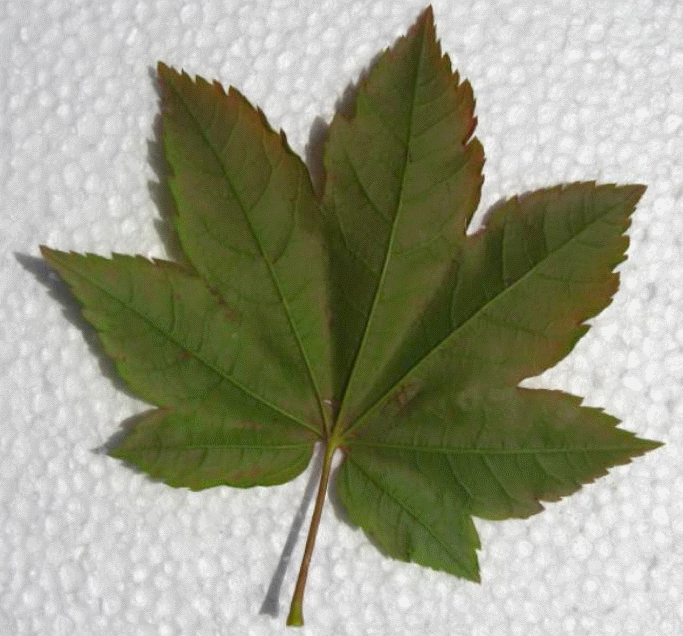
Figure $\PageIndex{1}$

A modification of this method would be to trace the shape onto a piece of graph paper and then count the number of squares completely inside the edge of the leaf to get a lower estimate of the area, and count the number of squares that touch the leaf to get an upper estimate of the area. If we repeat this process with smaller and smaller squares, we will have to do more counting and adding, but our estimates should be closer together — and closer to the actual area of the leaf.

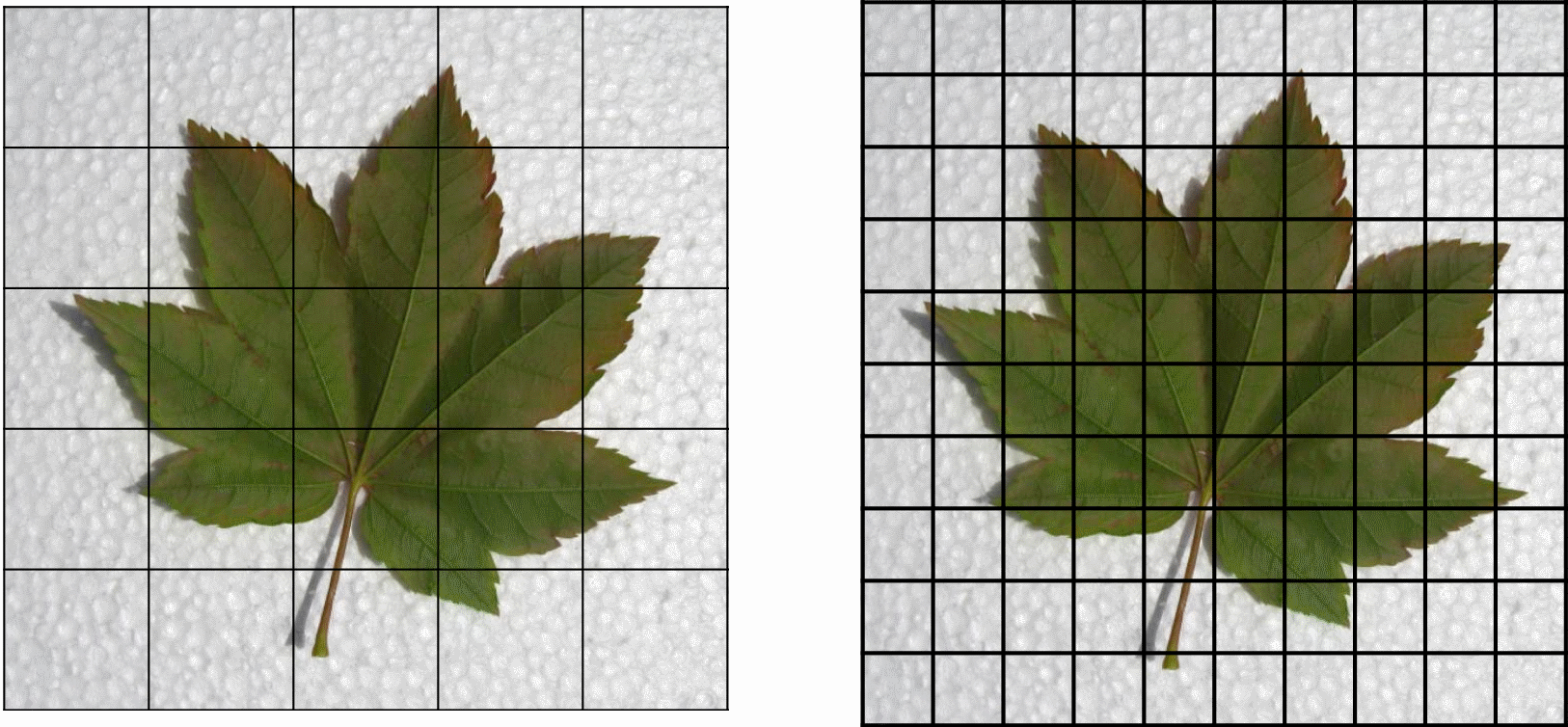
$On the left, a 5 by 5 square grid is superimposed on the leaf from the previous image; on the right, 10 by 10 grid is superimposed on the same leaf.$

Figure $\PageIndex{2}$

(We could also approximate the area of the leaf using a sheet of paper, scissors and an accurate scale. How?)

We can calculate the area $A$ between the graph of a function $y = f(x)$ and the $x$-axis by using similar methods.

$The graph of a function y = f(x) in the first quadrant with vertical lines at x = a and x = b, and the shaded region between these vertical lines, below the graph of the function and the positive x-axis labeled as A.$

We can divide the area into strips of width $w$ and determine the lower and upper values of $y = f(x)$ on each strip. Then we can approximate the area of each rectangle and add all of the little areas together to get $A_w$, an approximation of the exact area.

$The same graph as in the previous image, but with a square grid superimposed.$

The key idea is that if $w$ is small, then the rectangles are narrow, and the approximate area $A_w$ should be very close to the actual area $A$. If we take narrower and narrower rectangles, the approximate areas get closer and closer to the actual area: \[ A = \lim_{w \to 0} A_w\]The process described above is the basis for a technique called integration, and this part of calculus is called integral calculus. Integral calculus and integration will begin in Chapter 4. The process of taking the limit of a sum of “little” quantities will give us important information about a function and will also allow us to solve problems such as:

Find the length of the graph of $y = sin(x)$ over one period (from $x = 0$ to $x = 2\pi$).
Find the volume of a torus (“doughnut”) of radius 1 inch that has a hole of radius 2 inches.
A car starts at rest and has an acceleration of $5 + 3 \sin(t)$ feet per second per second in the northerly direction at time $t$ seconds. Where will the car be, relative to its starting position, after 100 seconds?

Problems

Approximate the area of the leaf in Figure $\PageIndex{2}$ using (a) the grid on the left. (b) the grid on the right.
A graph showing temperatures during the month of November appears below.
1. Approximate the shaded area between the temperature curve and the 65° line from Nov. 15 to Nov. 25.
2. The area of the “rectangle” is (base)(height) so what are the units of your answer in part (a)?
3. Approximate the shaded area between the temperature curve and the 65° line from Nov. 5 to Nov. 30.
4. Who might use or care about these results?
Describe a method for determining the volume of a compact fluorescent light bulb using a ruler, a large can, a scale and a jug of water.

A Unifying Process: Limits

We used similar processes to “solve” both the tangent line problem and the area problem. First, we found a way to get an approximate solution, and then we found a way to improve our approximation. Finally, we asked what would happen if we continued improving our approximations “forever”: that is, we “took a limit.”

For the tangent line problem, we let the point $Q$ get closer and closer and closer to $P$, the limit as $b$ approached $a$. In the area problem, we let the widths of the rectangles get smaller and smaller, the limit as $w$ approached $0$. Limiting processes underlie derivatives, integrals and several other fundamental topics in calculus, and we will examine limits and their properties in detail in Chapter 1.

Two Sides of the Same Coin: Differentiation and Integration

Just as the set-up of each of the two basic problems involved a limiting process, the solutions to the two problems are also related. The process of differentiation used to solve the tangent line problem and the process of integration used to solve the area problem turn out to be “opposites” of each other: each process undoes the effect of the other process. The Fundamental Theorem of Calculus in Chapter 4 will show how this “opposite” effect works.

Extensions of the Main Problems

The first five chapters present the two key ideas of calculus, show “easy” ways to calculate derivatives and integrals, and examine some of their applications. And there is more. Through the ensuing chapters, we will examine new functions and find ways to calculate their derivatives and integrals. We will extend the approximation ideas to use “easy” functions, such as polynomials, to approximate the values of “hard” functions, such as $sin(x)$ and $e^x$ . In later chapters, we will extend the notions of “tangent lines” and “areas” to 3-dimensional space as “tangent planes” and “volumes.”

Success in calculus will require time and effort on your part, but such a beautiful and powerful field is worth that time and effort.

Search

Text Color

Text Size

Margin Size

Font Type