5.7: Improper Integrals

In Section 5.4, we computed the work required to lift a payload of mass \(m\) from the surface of a moon of mass \(M\) and radius \(R\) to  a height \(H\) above the surface of the moon:\[\int_R^{R+H} \frac{GMm}{x^2}\, dx = \left[-\frac{GMm}{x}\right]_R^{R+H} = \frac{GMm}{R} - \frac{GMm}{R+H}\nonumber\]Notice that as the height \(H\) grows very large, the second term in this answer becomes very small and the total work approaches \(\displaystyle \frac{GMm}{R}\). We can write:\[\lim_{H \to \infty} \, \left[\frac{GMm}{R} - \frac{GMm}{R+H}\right] = \frac{GMm}{R}\nonumber\]Here we’re taking a limit of an expression that arose as the value of a definite integral, so we can also write:\[\frac{GMm}{R} = \lim_{H \to \infty} \, \left[\frac{GMm}{R} - \frac{GMm}{R+H}\right] = \lim_{H \to \infty} \, \int_R^{R+H} \frac{GMm}{x^2}\, dx\nonumber\]We could write this last integral, at least informally, as:\[\int_R^{\infty}  \frac{GMm}{x^2}\, dx\nonumber\]We call this new type of integral an improper integral because the interval of integration is infinite, violating an assumption we made when originally developing the definite integral \(\displaystyle \int_a^b f(x)\, dx\) using  Riemann sums that the length of the interval of integration, \(\left[a, b\right]\), was finite.

Example \(\PageIndex{1}\)

Represent the area of the infinite region between \(\displaystyle f(x) = \frac{1}{x^2}\) and the \(x\)-axis for \(x \geq 1\):

as an improper integral.

Solution

We can represent the area of region (which has infinite length) as:\[\int_1^{\infty} \frac{1}{x^2} \, dx\nonumber\]We don’t yet know whether this area is finite or infinite.

Practice \(\PageIndex{1}\)

Represent the volume swept out when the infinite region between \(\displaystyle f(x) = \frac{1}{x}\) and the \(x\)-axis for \(x \geq 4\) is revolved about the \(x\)-axis:

using an improper integral.

Answer

\(\displaystyle \int_4^{\infty} \pi\cdot \left(\frac{1}{x}\right)^2 \, dx = \pi \int_4^{\infty} \frac{1}{x^2} \, dx\)

General Strategy for Improper Integrals

In the lifting-a-payload example above, we defined our first improper integral as the limit of a “proper” integral over a finite interval as the length of the interval became larger and larger.

Our general approach to evaluate improper integrals over infinitely long intervals — as well as another type of improper integral introduced later in this section — will mimic this strategy: Shrink the interval of integration so you have a (proper) definite integral you can evaluate, then let the interval grow to approach the desired interval of integration. The value of the improper integral will be the limiting value of the (proper) definite integrals as the intervals grow to the interval you want, provided that this limit exists.

Infinitely Long Intervals of Integration

To evaluate an improper integral on an infinitely long interval:

• replace the infinitely long interval with a finite interval
• evaluate the integral on the finite interval
• let the finite interval grow longer and longer, approaching the original infinitely long interval

Example \(\PageIndex{2}\)

Evaluate \(\displaystyle \int_1^{\infty} \frac{1}{x^2}\, dx\):

Solution

The interval \([1, \infty)\) is infinitely long, but we can evaluate the integral on finite intervals such as \([1, 2]\), \([1, 10]\), \([1, 1000]\) and, more generally, \([1, M]\) where \(M\) is some massive positive number:
\begin{align*}
\int_1^2 \frac{1}{x^2}\ dx &= \left[-\frac{1}{x}\right]_1^{2} = \left[-\frac{1}{2}\right] - \left[-\frac{1}{1}\right] = 1 - \frac{1}{2} = \frac{1}{2}\\
\int_1^{10} \frac{1}{x^2}\ dx &= \left[-\frac{1}{x}\right]_1^{10} = \left[-\frac{1}{10}\right] - \left[-\frac{1}{1}\right] = 1 - \frac{1}{10} = \frac{9}{10}\\
\int_1^{1000} \frac{1}{x^2}\ dx &= \left[-\frac{1}{x}\right]_1^{1000} = \left[-\frac{1}{1000}\right] - \left[-\frac{1}{1}\right]  = 1 - \frac{1}{1000} = \frac{999}{1000}\end{align*}
and, more generally, \(\displaystyle \int_1^{M} \frac{1}{x^2}\, dx = 1 - \frac{1}{M}\) so:\[\int_1^{\infty} \frac{1}{x^2}\, dx = \lim_{M \to \infty} \, \int_1^M \frac{1}{x^2}\, dx  = \lim_{M \to \infty} \, \left[1 - \frac{1}{M}\right] = 1\nonumber\]The value of the improper integral is \(1\).

We say that the improper integral \(\displaystyle \int_1^{\infty} \frac{1}{x^2}\, dx\) in the Example 2 “is convergent” and that it “converges to \(1\).”

Furthermore, from Example 1, we know that this improper integral represents the area of an infinitely long region. We now have an example — which you may find highly counterintuitive — of a region with infinite length but finite area.

Not all improper integrals converge, however.

Example \(\PageIndex{3}\)

Evaluate each improper integral.

1. \(\displaystyle \int_0^{\infty} \frac{1}{1+x^2} \ dx\)
2. \(\displaystyle \int_1^{\infty} \frac{1}{x} \ dx\)
3. \(\displaystyle \int_{0}^{\infty} \cos(x) \, dx\)

See below for graphical interpretations of these integrals as areas of unbounded regions:

Solution

1. Replacing the upper limit of the improper integral with a massive positive number \(M\): \begin{align*}\int_0^{\infty} \frac{1}{1+x^2} \ dx &= \lim_{M\to \infty} \, \int_0^{M} \frac{1}{1+x^2} \ dx = \lim_{M\to \infty} \, \Big[\arctan(x)\Big]_0^M \\ &=  \lim_{M\to \infty} \, \Big[\arctan(M) - 0\Big] = \frac{\pi}{2}\end{align*} so the improper integral is convergent and converges to \(\displaystyle \frac{\pi}{2}\).
2. Replacing the upper limit of the improper integral with a massive positive number \(M\):\[\int_1^{\infty} \frac{1}{x} \ dx = \lim_{M\to \infty} \, \int_1^{M} \frac{1}{x} \ dx = \lim_{M\to \infty} \, \Big[\ln(x)\Big]_1^M =  \lim_{M\to \infty} \, \ln(M) = \infty\nonumber\]Because this limit diverges, we say the improper integral is divergent or that it diverges.
3. Once again replacing \(\infty\) with \(M\) in the upper limit of the integral:\[\lim_{M\to \infty} \, \int_0^{M} \cos(x) \, dx = \lim_{M\to \infty} \, \Big[\sin(x)\Big]_0^M =  \lim_{M\to \infty} \, \sin(M)\nonumber\]As \(M\) grows without bound, the values of \(\sin(M)\) oscillate between \(-1\) and \(1\), never approaching a single value, so the limit does not exist; we say that this improper integral diverges.

Practice \(\PageIndex{2}\)

Evaluate:

1. \(\displaystyle \int_1^{\infty} \frac{1}{x^3} \ dx\)
2. \(\displaystyle \int_{0}^{\infty} \sin(x) \, dx\)

Answer

1. \(\displaystyle \int_1^{\infty} \frac{1}{x^3} \ dx = \lim_{M\to \infty} \int_1^{M} x^{-3} \ dx = \lim_{M\to \infty} \left[-\frac12 x^{-2}\right]_1^M = \lim_{M\to \infty} \left[-\frac12 \cdot \frac{1}{M^2} + \frac12\right] = \frac12\)
2. Replacing \(\infty\) with \(M\) in the upper limit of the integral: \begin{align*}\int_0^{\infty} \sin(x) \ dx &= \lim_{M\to \infty} \int_0^{M} \sin(x) \ dx = \lim_{M\to \infty} \Big[-\cos(x)\Big]_0^M \\ &= \lim_{M\to \infty} \Big[-\cos(M)+1\Big] = \lim_{M\to \infty} \, [1-\cos(M)\end{align*} This limit does not exist (the values of \(1-\cos(M)\) oscillate between \(0\) and \(2\) and never approach any fixed number) so the improper integral diverges.

Definition

For any integrable function \(f(x)\) defined for all \(x \geq a\) and any integrable function \(g(x)\) defined for all \(x \leq b\):
\begin{align*}
\int_a^{\infty} f(x) \, dx &= \lim_{M\to \infty} \, \int_a^M f(x) \, dx\\
\int_{-\infty}^b g(x) \, dx &= \lim_{N\to -\infty} \, \int_N^b g(x) \, dx
\end{align*}

If the limit in question exists and is finite, we say that the corresponding improper integral converges or is convergent and define the value of the improper integral to be the value of the limit. If the limit in question does not exist, we say that the corresponding improper integral diverges or is divergent.

Functions Undefined at an Endpoint of the Interval of Integration

Consider the graph of \(\frac{1}{\sqrt{x}}\) on the interval \((0,1]\):

and compare this region to the graph from Example 2. It appears we can generate the new region by reflecting the old region across \(y = x\) and adding a rectangle (of area \(1\)) at the bottom, so we might reasonably assume that the integral \(\int_0^1 \frac{1}{\sqrt{x}} \, dx\) is a finite number. This integral is over a finite interval, \([0,1]\), but we have a new problem: the integrand is undefined at \(x = 0\), one of the endpoints of the interval of integration. This violates another assumption we made when developing the definition of a definite integral as a limit of Riemann sums.

If the function you want to integrate is unbounded at one of the endpoints of an interval of finite length, as in this situation, you can shrink the interval of integration so that the function is bounded at both endpoints of the new, smaller interval, then evaluate the integral over the smaller interval, and finally let the smaller interval grow to approach the original interval.

Example \(\PageIndex{4}\)

Evaluate \(\displaystyle \int_0^1 \frac{1}{\sqrt{x}} \, dx\).

Solution

The function \(\displaystyle \frac{1}{\sqrt{x}}\) is not defined at \(x = 0\), the lower endpoint of integration, but the function is bounded on intervals such as \([0.36, 1]\), \([0.09, 1]\) and, more generally, on the interval \([c , 1]\) for any \( c > 0\):
\begin{align*}
\int_{0.36}^1 \frac{1}{\sqrt{x}}\ dx &= \Big[2\sqrt{x}\,\Big]_{0.36}^{1} = 2\sqrt{1}-2\sqrt{0.36} = 2 - 1.2 = 0.8\\
\int_{0.09}^1 \frac{1}{\sqrt{x}}\ dx &= \Big[2\sqrt{x}\,\Big]_{0.09}^{1} = 2\sqrt{1}-2\sqrt{0.09} = 2 - 0.6 = 1.4 \end{align*}
and, in general:\[\int_{c}^1 \frac{1}{\sqrt{x}}\ dx = \Big[2\sqrt{x}\,\Big]_{c}^{1} = 2\sqrt{1}-2\sqrt{c} = 2-2\sqrt{c}\nonumber\]so, taking the limit as \(c\) decreases toward \(0\):\[\lim_{c\to 0^{+}} \, \int_{c}^1 \frac{1}{\sqrt{x}}\ dx = \lim_{c\to 0^{+}} \, \left[\, 2-2\sqrt{c}\, \right] = 2\nonumber\]which is what you should have expected based on the graph.

NOTE SOMEWHERE A region of area \(1\) plus a rectangle of area \(1\) should have an area of \(1+1=2\).

Definition

For any function \(f(x)\) defined and continuous on \((a,b]\) and any function \(g(x)\) defined and continuous on \([a,b)\):
\begin{align*}
\int_a^{b} f(x) \, dx &= \lim_{c\to a^{+}} \, \int_c^b f(x) \, dx\\
\int_a^{b} g(x) \, dx &= \lim_{c\to b^{-}} \, \int_a^c g(x) \, dx
\end{align*}

If the limit exists, we say the integral converges and define the value of the integral to be the value of the limit. If the limit does not exist, we say that the integral diverges.

Practice \(\PageIndex{3}\)

Show that:

1. \(\displaystyle \int_1^{10} \frac{1}{\sqrt{10-x}}\, dx = 6\) and
2. \(\displaystyle \int_0^{1} \frac{1}{x}\, dx\) diverges.

Answer

1. The integral is improper at its upper limit, where \(x=10\), so: \begin{align*}\int_1^{10} \frac{1}{\sqrt{10-x}} \ dx &= \lim_{c\to 10^{-}} \int_1^{c} \left(10-x\right)^{-\frac12} \ dx = \lim_{c\to 10^{-}} \left[-2\sqrt{10-x}\right]_1^c \\ &= \lim_{c\to 10^{-}} \left[-2\sqrt{10-c}+2\sqrt{9}\right] = 0+2\cdot 3 = 6\end{align*}
2. The integral is improper at its lower limit, where \(x=0\), so:\[\int_0^{1} \frac{1}{x} \ dx = \lim_{c\to 0^{+}} \int_c^{1} \frac{1}{x} \ dx = \lim_{c\to 0^{+}} \Big[\ln\left(\left|x\right|\right)\Big]_c^1 = \lim_{c\to 0^{+}} \left[\ln(1)-\ln(c)\right] = \infty\]so the integral diverges.

If an integrand is unbounded at one or more points inside the interval of integration, you can split the original improper integral into two or more improper integrals over subintervals where the integrand is unbounded at only one endpoint of each subinterval. (See Problems 22–26 for practice with integrals of this type.)

Testing for Convergence: The P-Test and the Comparison Test

Sometimes we care only whether or not an improper integral converges. We now consider two methods for testing the convergence of an improper integral. Neither method gives you the actual value of the integral, but each enables you to determine whether or not certain improper integrals converge. The Comparison Test for Integrals enables you to determine the convergence (or divergence) of certain integrals by comparing them with other (easier) integrals. The P-Test involves special cases often used with the Comparison Test for Integrals.

P-Test for integrals

For any \(a > 0\), the improper integral \(\displaystyle \int_a^{\infty} \frac{1}{x^p}\, dx\) converges if \(p > 1\) and diverges if \(p \leq 1\).

Proof

It is easiest to consider three cases rather than two: \(p = 1\), \(p > 1\) and \(p < 1\). If \(p=1\) then:
\begin{align*}\int_a^{\infty} \frac{1}{x^p}\, dx &= \int_a^{\infty} \frac{1}{x}\, dx = \lim_{M\to\infty}\, \int_a^M \frac{1}{x}\, dx = \lim_{M\to\infty}\,\Big[\ln\left(\left|x\right|\right)\Big]_a^M \\
&= \lim_{M\to\infty}\,\Big[\ln(M) - \ln(a)\Big] = \infty\end{align*}
so the improper integral diverges. For the other two cases, \(p \neq 1\), so:\[\lim_{M\to\infty}\, \int_a^M x^{-p}\, dx = \lim_{M\to\infty}\,\left[\frac{x^{-p+1}}{-p+1}\right]_a^M = \lim_{M\to\infty}\,\left[\frac{M^{1-p}}{1-p} - \frac{a^{1-p}}{1-p}\right]\nonumber\]If \(p > 1\), then \(1 - p < 0\) so \(\displaystyle \lim_{M\to\infty}\, \frac{M^{1-p}}{1-p} = 0\) and:\[\int_a^{\infty} \frac{1}{x^p}\, dx = \lim_{M\to\infty}\,\left[\frac{M^{-p+1}}{-p+1} - \frac{a^{-p+1}}{-p+1}\right] = \frac{a^{1-p}}{p-1}\nonumber\]which is a finite number, so the improper integral converges. If \(p < 1\), then \(1 - p > 0\) so \(\displaystyle \lim_{M\to\infty}\, \frac{M^{1-p}}{1-p} = \infty\) and: \[\int_a^{\infty} \frac{1}{x^p}\, dx = \lim_{M\to\infty}\,\left[\frac{M^{-p+1}}{-p+1} - \frac{a^{-p+1}}{-p+1}\right] = \infty\nonumber\]so the improper integral diverges.

Example \(\PageIndex{5}\)

Determine the convergence or divergence of each integral:

1. \(\displaystyle \int_5^{\infty} \frac{1}{x^2}\, dx\)
2. \(\displaystyle \int_1^{\infty} \frac{1}{\sqrt{x}}\, dx\)
3. \(\displaystyle \int_1^{8} \frac{1}{\sqrt[3]{x}}\, dx\)

Solution

1. The integral matches the form required by the P-Test with \(p = 2 > 1\), so the improper integral converges. The P-Test does not tell us the value of the integral.
2. The integral matches the form required by the P-Test with \(p = \frac12 < 1\), so the improper integral diverges.
3. This is not an improper integral, so the P-Test does not apply, but:\[\int_1^{8} \frac{1}{\sqrt[3]{x}}\, dx = \int_1^8 x^{-\frac13}\, dx = \left[\frac32 x^{\frac23}\right]_1^8 = \frac32\left[8^{\frac23}-1^{\frac23}\right] = \frac32\left[4-1\right] = \frac92\nonumber\]so the value of the integral is \(4.5\).

The following Comparison Test enables us to determine the convergence or divergence of an improper integral of a positive function by comparing this function with functions whose improper integrals we already know converge or diverge.

Comparison Test for Integrals of Positive Functions

Suppose \(f(x)\) and \(g(x)\) are defined and integrable for all \(x \geq a\) with \(0 \leq f(x) \leq g(x)\). Then:

• \(\displaystyle \int_a^{\infty} g(x)\, dx\) converges \(\displaystyle \ \Rightarrow \ \ \int_a^{\infty} f(x)\, dx\) converges.
• \(\displaystyle \int_a^{\infty} f(x)\, dx\) diverges \(\displaystyle \ \Rightarrow \ \int_a^{\infty} g(x)\, dx\) diverges.

The proof involves a straightforward application of the definition of an improper integral and various facts about limits, but the graph below provides a geometrically intuitive way of understanding why these results must hold:

If \(\int_a^{\infty} g(x)\, dx\) converges, then the area under the graph of \(g(x)\) is finite, so the (smaller) area under the graph of \(f(x)\) must also be finite, and \(\int_a^{\infty} f(x)\, dx\) must converge as well. If \(\int_a^{\infty} f(x)\, dx\) diverges, then the area under the graph of \(f(x)\) is infinite, so the (bigger) area under the graph of \(g(x)\) must also be infinite, and \(\int_a^{\infty} g(x)\, dx\) must also diverge.

Just as important as understanding what this Comparison Test does tell us is realizing what the Comparison Test does not tell us. If \(\int_a^{\infty} g(x)\, dx\) diverges, or if \(\int_a^{\infty} f(x)\, dx\) converges, the Comparison Test tells us absolutely nothing about the convergence or divergence of the other integral. Geometrically, if \(\int_a^{\infty} g(x)\, dx\) diverges, then the area under the graph of \(g(x)\) is infinite, but the (smaller) area under the graph of \(f(x)\) could be either finite or infinite, so we can't conclude anything about the convergence or divergence of \(\int_a^{\infty} f(x)\, dx\). Likewise, if \(\int_a^{\infty} f(x)\, dx\) converges, then the area under the graph of \(f(x)\) is finite, but the (bigger) area under the graph of \(g(x)\) could be either finite or infinite, so we can't conclude anything about the convergence or divergence of \(\int_a^{\infty} g(x)\, dx\). 

Example \(\PageIndex{6}\)

Determine whether each of these integrals is convergent or divergent by comparing it with an appropriate integral that you already know converges or diverges:

1. \(\displaystyle \int_1^{\infty} \frac{7}{x^3+5}\, dx\)
2. \(\displaystyle \int_1^{\infty} \frac{3+\sin(x)}{x^2}\, dx\)
3. \(\displaystyle \int_6^{\infty} \frac{9}{\sqrt{x-5}}\, dx\)

Solution

1. We know that \(5 > 0\) and \(x \geq 1\) so:\[x^3+5 > x^3 \ \Rightarrow \ 0 < \frac{1}{x^3+5} < \frac{1}{x^3} \ \Rightarrow \ 0 < \frac{7}{x^3+5} < \frac{7}{x^3}\nonumber\]We also know, by the P-Test with \(p = 3 >1\), that \(\displaystyle \int_1^{\infty} \frac{1}{x^3} \, dx\) converges, so  \(\displaystyle \int_1^{\infty} \frac{7}{x^3} \, dx = 7\cdot \int_1^{\infty} \frac{1}{x^3} \, dx\) also converges. By the Comparison Test, the smaller integral \(\displaystyle \int_1^{\infty} \frac{7}{x^3+5} \, dx\) must converge as well. (The numerator of the original integrand is constant and the dominant term in the denominator of that integrand is \(x^3\), so it should make sense to compare the original integrand with \(\displaystyle \frac{1}{x^3}\).)
2. We know that \(-1 \leq \sin(x) \leq 1\), so:\[2 \leq 3+\sin(x) \leq 4 \ \Rightarrow \ 0 < \frac{3+\sin(x)}{x^2} \leq \frac{4}{x^2} = 4\cdot \frac{1}{x^2}\nonumber\]By the P-Test with \(p = 2 >1\), \(\displaystyle \int_1^{\infty} \frac{1}{x^2} \, dx\) converges, so  \(\displaystyle \int_1^{\infty} \frac{4}{x^2} \, dx = 4\cdot \int_1^{\infty} \frac{1}{x^2} \, dx\) also converges. By the Comparison Test, the smaller integral \(\displaystyle \int_1^{\infty} \frac{3+\sin(x)}{x^2} \, dx\) must converge as well. (The numerator of the original integrand fluctuates between \(2\) and \(4\) while the dominant (and only) term in its denominator is \(x^2\), so it should make sense to compare the original integrand with \(\displaystyle \frac{1}{x^2}\).)
3. We know that \(\sqrt{u}\) is an increasing function, so:\[x-5 < x \ \Rightarrow \ \sqrt{x-5} < \sqrt{x} \ \Rightarrow \frac{1}{\sqrt{x-5}} > \frac{1}{\sqrt{x}}\nonumber\]By the P-Test with \(p = \frac12 < 1\), \(\displaystyle \int_6^{\infty} \frac{1}{\sqrt{x}} \, dx\) diverges, so the bigger integral \(\displaystyle \int_6^{\infty} \frac{1}{\sqrt{x-5}} \, dx\) must also diverge.

Problems

In Problems 1–26, evaluate each improper integral, or show why it diverges.

1. \(\displaystyle \int_{10}^{\infty} \frac{1}{x^3}\ dx\)
2. \(\displaystyle \int_{e}^{\infty} \frac{5}{x\cdot\left[\ln(x)\right]^2}\ dx\)
3. \(\displaystyle \int_{\sqrt{3}}^{\infty} \frac{1}{1+x^2}\ dx\)
4. \(\displaystyle \int_{1}^{\infty} \frac{2}{e^x}\ dx\)
5. \(\displaystyle \int_{e}^{\infty} \frac{5}{x\cdot\ln(x)}\ dx\)
6. \(\displaystyle \int_{0}^{\infty} \frac{x}{1+x^2}\ dx\)
7. \(\displaystyle \int_{3}^{\infty} \frac{1}{x-2}\ dx\)
8. \(\displaystyle \int_{3}^{\infty} \frac{1}{(x-2)^2}\ dx\)
9. \(\displaystyle \int_{3}^{\infty} \frac{1}{(x-2)^3}\ dx\)
10. \(\displaystyle \int_{3}^{\infty} \frac{1}{x+2}\ dx\)
11. \(\displaystyle \int_{3}^{\infty} \frac{1}{(x+2)^2}\ dx\)
12. \(\displaystyle \int_{3}^{\infty} \frac{1}{(x+2)^3}\ dx\)
13. \(\displaystyle \int_{0}^{4} \frac{1}{\sqrt{x}}\ dx\)
14. \(\displaystyle \int_{0}^{8} \frac{1}{\sqrt[3]{x}}\ dx\)
15. \(\displaystyle \int_{0}^{16} \frac{1}{\sqrt[4]{x}}\ dx\)
16. \(\displaystyle \int_{0}^{2} \frac{1}{\sqrt{2-x}}\ dx\)
17. \(\displaystyle \int_{0}^{2} \frac{1}{\sqrt{4-x^2}}\ dx\)
18. \(\displaystyle \int_{0}^{2} \frac{3x^2}{\sqrt{8-x^3}}\ dx\)
19. \(\displaystyle \int_{-2}^{\infty} \sin(x) \ dx\)
20. \(\displaystyle \int_{\pi}^{\infty} \sin(x) \ dx\)
21. \(\displaystyle \int_{0}^{\frac{\pi}{2}} \tan(x) \ dx\)
22. \(\displaystyle \int_{0}^{3} \frac{1}{x-2}\ dx\)
23. \(\displaystyle \int_{0}^{\pi} \tan(x) \ dx\)
24. \(\displaystyle \int_{3}^{\infty} \frac{1}{x\sqrt{x}} \ dx\)
25. \(\displaystyle \int_{-\infty}^{\infty} \frac{1}{x^2+1} \ dx\)
26. \(\displaystyle \int_{-\infty}^{0} \frac{1}{x^2} \ dx\)

In Problems 27–44, determine whether each improper integral converges or diverges, but do not evaluate the integral.

27. \(\displaystyle \int_{1}^{\infty} \frac{1}{x^5} \ dx\)
28. \(\displaystyle \int_{2}^{\infty} \frac{1}{\sqrt[5]{x}} \ dx\)
29. \(\displaystyle \int_{3}^{\infty} \frac{1}{\sqrt[5]{x^6}} \ dx\)
30. \(\displaystyle \int_{4}^{\infty} \frac{1}{\sqrt[5]{x^4}} \ dx\)
31. \(\displaystyle \int_{5}^{\infty} \frac{1}{\sqrt{x \sqrt[3]{x}}} \ dx\)
32. \(\displaystyle \int_{6}^{\infty} x^{-\frac47} \ dx\)
33. \(\displaystyle \int_{7}^{\infty} x^{-\frac74} \ dx\)
34. \(\displaystyle \int_{8}^{\infty} \frac{1}{1+x^2} \ dx\)
35. \(\displaystyle \int_{3}^{\infty} \frac{1}{x^2+5} \ dx\)
36. \(\displaystyle \int_{4}^{\infty} \frac{7}{x^2+5} \ dx\)
37. \(\displaystyle \int_{5}^{\infty} \frac{1}{x^3+x} \ dx\)
38. \(\displaystyle \int_{6}^{\infty} \frac{1}{x-2} \ dx\)
39. \(\displaystyle \int_{e}^{\infty} \frac{7}{x+\ln(x)} \ dx\)
40. \(\displaystyle \int_{2}^{\infty} \frac{1}{x^2-1} \ dx\)
41. \(\displaystyle \int_{\pi}^{\infty} \frac{1+\cos(x)}{x^2} \ dx\)
42. \(\displaystyle \int_{0}^{\infty} \frac{x^4}{x^6+1} \ dx\)
43. \(\displaystyle \int_{0}^{\infty} \frac{x^4}{x^5+1} \ dx\)
44. \(\displaystyle \int_{0}^{\infty} \frac{\sqrt{x}}{x^2+1} \ dx\)
45. Example 3(b) showed that \(\displaystyle \int_1^M \frac{1}{x}\ dx\) grew arbitrarily large as \(M\) grew arbitrarily large, so no finite amount of paint would cover the region bounded by the \(x\)-axis and the graph of \(\displaystyle f(x) = \frac{1}{x}\) for \(x > 1\):
    
    Show that the volume of the solid obtained when the region graphed above is revolved about the \(x\)-axis:
    
    is finite, so the 3-dimensional trumpet-shaped region can be filled with a finite amount of paint. Does this present a contradiction?
46. Determine whether or not the volume of the solid obtained by revolving the region between the \(x\)-axis and the graph of \(\displaystyle f(x) = \frac{\sin(x)}{x}\) for for \(x \geq 1\):
    
    about the \(x\)-axis is finite.
47. Compute the volume of the solid obtained when the region in the first quadrant between the positive \(x\)-axis and the graph of \(\displaystyle f(x) = \frac{1}{x^2 + 1}\):
    
    is revolved about the \(x\)-axis.
48. Compute the volume of the solid obtained when the region in the first quadrant between the positive \(x\)-axis and the graph of \(\displaystyle f(x) = e^{-x}\) is revolved about the \(x\)-axis.
49. Compute the volume of the solid obtained when the region in the first quadrant between the positive \(x\)-axis and the graph of \(\displaystyle f(x) = \frac{1}{x^2 + 1}\):
    
    is revolved about the \(y\)-axis.
50. Compute the volume of the solid obtained when the region in the first quadrant between the positive \(x\)-axis and the graph of \(\displaystyle f(x) = e^{-x}\) is revolved about the \(y\)-axis.
51. Use the figure below left to help determine which is larger: \(\displaystyle \int_1^A \frac{1}{x} \ dx\) or \(\displaystyle \sum_{k=1}^{A-1} \, \frac{1}{k}\).
    
52. Use the figure above right to help determine which is larger: \(\displaystyle \int_1^A \frac{1}{x} \ dx\) or \(\displaystyle \sum_{k=2}^{A} \, \frac{1}{k}\).
53. Use the figure below left to help determine which is larger: \(\displaystyle \int_1^A \frac{1}{x^2} \ dx\) or \(\displaystyle \sum_{k=1}^{A-1} \, \frac{1}{k^2}\).
    
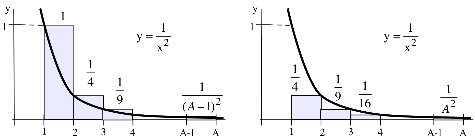
54. Use the figure above right to help determine which is larger: \(\displaystyle \int_1^A \frac{1}{x^2} \ dx\) or \(\displaystyle \sum_{k=2}^{A} \, \frac{1}{k^2}\).

The Laplace transform of a function \(f(t)\) is defined using an improper integral involving a parameter \(s\):\[F(s) = \int_0^{\infty} e^{-st}\cdot f(t) \ dt\nonumber\]Laplace transforms are often used to solve differential equations.

55. Compute the Laplace transform of the constant function \(f(t) = 1\).
56. Compute the Laplace transform of \(f(t) = e^{4t}\).
57. Define a function \(g(t)\) by:\[g(t) = \left\{ \begin{array}{rl} { 0 } & { \text{if } t < 2 } \\ { 1 } & { \text{if } t \geq 2 } \end{array}\right.\nonumber\]Compute the Laplace transform of \(g(t)\).
58. Define a function \(h(t)\) by:\[h(t) = \left\{ \begin{array}{rl} { 1 } & { \text{if } t < 3 } \\ { 0 } & { \text{if } t \geq 3 } \end{array}\right.\nonumber\]Compute the Laplace transform of \(h(t)\).
59. Devise a “Q-Test” to determine whether \(\displaystyle \int_0^b \frac{1}{x^q}\ dx\) converges or diverges for any number \(b > 0\).
60. Use the result of the previous Problem to test the convergence of \(\displaystyle \int_0^e \frac{1}{\sqrt[3]{x}}\ dx\) and \(\displaystyle \int_0^{\pi} \frac{1}{x\cdot \sqrt[3]{x}}\ dx\).