
3.6: Surface Area
- Page ID
- 166232
\( \newcommand{\vecs}[1]{\overset { \scriptstyle \rightharpoonup} {\mathbf{#1}} } \)
\( \newcommand{\vecd}[1]{\overset{-\!-\!\rightharpoonup}{\vphantom{a}\smash {#1}}} \)
\( \newcommand{\dsum}{\displaystyle\sum\limits} \)
\( \newcommand{\dint}{\displaystyle\int\limits} \)
\( \newcommand{\dlim}{\displaystyle\lim\limits} \)
\( \newcommand{\id}{\mathrm{id}}\) \( \newcommand{\Span}{\mathrm{span}}\)
( \newcommand{\kernel}{\mathrm{null}\,}\) \( \newcommand{\range}{\mathrm{range}\,}\)
\( \newcommand{\RealPart}{\mathrm{Re}}\) \( \newcommand{\ImaginaryPart}{\mathrm{Im}}\)
\( \newcommand{\Argument}{\mathrm{Arg}}\) \( \newcommand{\norm}[1]{\| #1 \|}\)
\( \newcommand{\inner}[2]{\langle #1, #2 \rangle}\)
\( \newcommand{\Span}{\mathrm{span}}\)
\( \newcommand{\id}{\mathrm{id}}\)
\( \newcommand{\Span}{\mathrm{span}}\)
\( \newcommand{\kernel}{\mathrm{null}\,}\)
\( \newcommand{\range}{\mathrm{range}\,}\)
\( \newcommand{\RealPart}{\mathrm{Re}}\)
\( \newcommand{\ImaginaryPart}{\mathrm{Im}}\)
\( \newcommand{\Argument}{\mathrm{Arg}}\)
\( \newcommand{\norm}[1]{\| #1 \|}\)
\( \newcommand{\inner}[2]{\langle #1, #2 \rangle}\)
\( \newcommand{\Span}{\mathrm{span}}\) \( \newcommand{\AA}{\unicode[.8,0]{x212B}}\)
\( \newcommand{\vectorA}[1]{\vec{#1}} % arrow\)
\( \newcommand{\vectorAt}[1]{\vec{\text{#1}}} % arrow\)
\( \newcommand{\vectorB}[1]{\overset { \scriptstyle \rightharpoonup} {\mathbf{#1}} } \)
\( \newcommand{\vectorC}[1]{\textbf{#1}} \)
\( \newcommand{\vectorD}[1]{\overrightarrow{#1}} \)
\( \newcommand{\vectorDt}[1]{\overrightarrow{\text{#1}}} \)
\( \newcommand{\vectE}[1]{\overset{-\!-\!\rightharpoonup}{\vphantom{a}\smash{\mathbf {#1}}}} \)
\( \newcommand{\vecs}[1]{\overset { \scriptstyle \rightharpoonup} {\mathbf{#1}} } \)
\(\newcommand{\longvect}{\overrightarrow}\)
\( \newcommand{\vecd}[1]{\overset{-\!-\!\rightharpoonup}{\vphantom{a}\smash {#1}}} \)
\(\newcommand{\avec}{\mathbf a}\) \(\newcommand{\bvec}{\mathbf b}\) \(\newcommand{\cvec}{\mathbf c}\) \(\newcommand{\dvec}{\mathbf d}\) \(\newcommand{\dtil}{\widetilde{\mathbf d}}\) \(\newcommand{\evec}{\mathbf e}\) \(\newcommand{\fvec}{\mathbf f}\) \(\newcommand{\nvec}{\mathbf n}\) \(\newcommand{\pvec}{\mathbf p}\) \(\newcommand{\qvec}{\mathbf q}\) \(\newcommand{\svec}{\mathbf s}\) \(\newcommand{\tvec}{\mathbf t}\) \(\newcommand{\uvec}{\mathbf u}\) \(\newcommand{\vvec}{\mathbf v}\) \(\newcommand{\wvec}{\mathbf w}\) \(\newcommand{\xvec}{\mathbf x}\) \(\newcommand{\yvec}{\mathbf y}\) \(\newcommand{\zvec}{\mathbf z}\) \(\newcommand{\rvec}{\mathbf r}\) \(\newcommand{\mvec}{\mathbf m}\) \(\newcommand{\zerovec}{\mathbf 0}\) \(\newcommand{\onevec}{\mathbf 1}\) \(\newcommand{\real}{\mathbb R}\) \(\newcommand{\twovec}[2]{\left[\begin{array}{r}#1 \\ #2 \end{array}\right]}\) \(\newcommand{\ctwovec}[2]{\left[\begin{array}{c}#1 \\ #2 \end{array}\right]}\) \(\newcommand{\threevec}[3]{\left[\begin{array}{r}#1 \\ #2 \\ #3 \end{array}\right]}\) \(\newcommand{\cthreevec}[3]{\left[\begin{array}{c}#1 \\ #2 \\ #3 \end{array}\right]}\) \(\newcommand{\fourvec}[4]{\left[\begin{array}{r}#1 \\ #2 \\ #3 \\ #4 \end{array}\right]}\) \(\newcommand{\cfourvec}[4]{\left[\begin{array}{c}#1 \\ #2 \\ #3 \\ #4 \end{array}\right]}\) \(\newcommand{\fivevec}[5]{\left[\begin{array}{r}#1 \\ #2 \\ #3 \\ #4 \\ #5 \\ \end{array}\right]}\) \(\newcommand{\cfivevec}[5]{\left[\begin{array}{c}#1 \\ #2 \\ #3 \\ #4 \\ #5 \\ \end{array}\right]}\) \(\newcommand{\mattwo}[4]{\left[\begin{array}{rr}#1 \amp #2 \\ #3 \amp #4 \\ \end{array}\right]}\) \(\newcommand{\laspan}[1]{\text{Span}\{#1\}}\) \(\newcommand{\bcal}{\cal B}\) \(\newcommand{\ccal}{\cal C}\) \(\newcommand{\scal}{\cal S}\) \(\newcommand{\wcal}{\cal W}\) \(\newcommand{\ecal}{\cal E}\) \(\newcommand{\coords}[2]{\left\{#1\right\}_{#2}}\) \(\newcommand{\gray}[1]{\color{gray}{#1}}\) \(\newcommand{\lgray}[1]{\color{lightgray}{#1}}\) \(\newcommand{\rank}{\operatorname{rank}}\) \(\newcommand{\row}{\text{Row}}\) \(\newcommand{\col}{\text{Col}}\) \(\renewcommand{\row}{\text{Row}}\) \(\newcommand{\nul}{\text{Nul}}\) \(\newcommand{\var}{\text{Var}}\) \(\newcommand{\corr}{\text{corr}}\) \(\newcommand{\len}[1]{\left|#1\right|}\) \(\newcommand{\bbar}{\overline{\bvec}}\) \(\newcommand{\bhat}{\widehat{\bvec}}\) \(\newcommand{\bperp}{\bvec^\perp}\) \(\newcommand{\xhat}{\widehat{\xvec}}\) \(\newcommand{\vhat}{\widehat{\vvec}}\) \(\newcommand{\uhat}{\widehat{\uvec}}\) \(\newcommand{\what}{\widehat{\wvec}}\) \(\newcommand{\Sighat}{\widehat{\Sigma}}\) \(\newcommand{\lt}{<}\) \(\newcommand{\gt}{>}\) \(\newcommand{\amp}{&}\) \(\definecolor{fillinmathshade}{gray}{0.9}\)- Find the parametric representations of a cylinder, a cone, and a sphere.
- Describe the surface area of a parametric surface.
We have seen that a line integral is an integral over a path in a plane or in space. However, if we wish to integrate over a surface (a two-dimensional object) rather than a path (a one-dimensional object) in space, then we need a new kind of integral that can handle integration over objects in higher dimensions. We can extend the concept of a line integral to a surface integral to allow us to perform this integration.
Surface integrals are important for the same reasons that line integrals are important. They have many applications to physics and engineering, and they allow us to develop higher dimensional versions of the Fundamental Theorem of Calculus. In particular, surface integrals allow us to generalize Green’s theorem to higher dimensions, and they appear in some important theorems we discuss in later sections.
Parametric Surfaces
A surface integral is similar to a line integral, except the integration is done over a surface rather than a path. In this sense, surface integrals expand on our study of line integrals. Just as with line integrals, there are two kinds of surface integrals: a surface integral of a scalar-valued function and a surface integral of a vector field.
However, before we can integrate over a surface, we need to consider the surface itself. Recall that to calculate a scalar or vector line integral over curve \(C\), we first need to parameterize \(C\). In a similar way, to calculate a surface integral over surface \(S\), we need to parameterize \(S\). That is, we need a working concept of a parameterized surface (or a parametric surface), in the same way that we already have a concept of a parameterized curve.
A parameterized surface is given by a description of the form
\[\mathbf{r}(u,v) = \langle x (u,v), \, y(u,v), \, z(u,v)\rangle.\]
Notice that this parameterization involves two parameters, \(u\) and \(v\), because a surface is two-dimensional, and therefore two variables are needed to trace out the surface. The parameters \(u\) and \(v\) vary over a region called the parameter domain, or parameter space—the set of points in the \(uv\)-plane that can be substituted into \(\mathbf r\). Each choice of \(u\) and \(v\) in the parameter domain gives a point on the surface, just as each choice of a parameter \(t\) gives a point on a parameterized curve. The entire surface is created by making all possible choices of \(u\) and \(v\) over the parameter domain.
Given a parameterization of surface
\[\mathbf{r}(u,v) = \langle x (u,v), \, y(u,v), \, z(u,v)\rangle.\]
the parameter domain of the parameterization is the set of points in the \(uv\)-plane that can be substituted into \(\mathbf r\).
Describe surface \(S\) parameterized by
\[\mathbf{r}(u,v) = \langle \cos u, \, \sin u, \, v \rangle, \, -\infty < u < \infty, \, -\infty < v < \infty. \nonumber\]
Solution
To get an idea of the shape of the surface, we first plot some points. Since the parameter domain is all of \(\mathbb{R}^2\), we can choose any value for u and v and plot the corresponding point. If \(u = v = 0\), then \(\mathbf r(0,0) = \langle 1,0,0 \rangle\), so point (1, 0, 0) is on \(S\). Similarly, points \(\mathbf r(\pi, 2) = (-1,0,2)\) and \(\mathbf r \left(\dfrac{\pi}{2}, 4\right) = (0,1,4)\) are on \(S\).
Although plotting points may give us an idea of the shape of the surface, we usually need quite a few points to see the shape. Since it is time-consuming to plot dozens or hundreds of points, we use another strategy. To visualize \(S\), we visualize two families of curves that lie on \(S\). In the first family of curves we hold \(u\) constant; in the second family of curves we hold \(v\) constant. This allows us to build a “skeleton” of the surface, thereby getting an idea of its shape.
- Suppose that \(u\) is a constant \(K\). Then the curve traced out by the parameterization is \(\langle \cos K, \, \sin K, \, v \rangle \), which gives a vertical line that goes through point \((\cos K, \sin K, v \rangle\) in the \(xy\)-plane.
- Suppose that \(v\) is a constant \(K\). Then the curve traced out by the parameterization is \(\langle \cos u, \, \sin u, \, K \rangle \), which gives a circle in plane \(z = K\) with radius 1 and center \((0, 0, K)\).
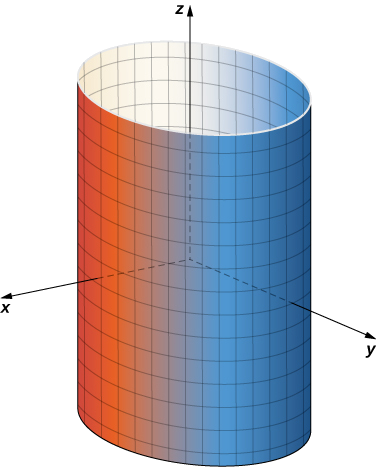
If \(u\) is held constant, then we get vertical lines; if \(v\) is held constant, then we get circles of radius 1 centered around the vertical line that goes through the origin. Therefore the surface traced out by the parameterization is cylinder \(x^2 + y^2 = 1\) (Figure \(\PageIndex{1}\)).
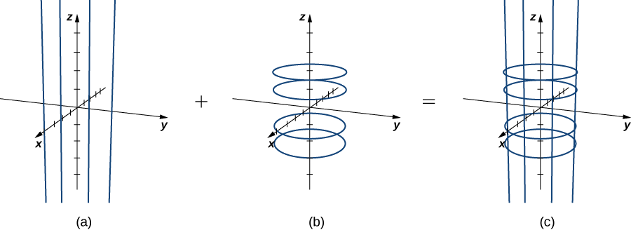
Notice that if \(x = \cos u\) and \(y = \sin u\), then \(x^2 + y^2 = 1\), so points from S do indeed lie on the cylinder. Conversely, each point on the cylinder is contained in some circle \(\langle \cos u, \, \sin u, \, k \rangle \) for some \(k\), and therefore each point on the cylinder is contained in the parameterized surface (Figure \(\PageIndex{2}\)).
Analysis
Notice that if we change the parameter domain, we could get a different surface. For example, if we restricted the domain to \(0 \leq u \leq \pi, \, -\infty < v < 6\), then the surface would be a half-cylinder of height 6.
Describe the surface with parameterization
\[\mathbf{r} (u,v) = \langle 2 \, \cos u, \, 2 \, \sin u, \, v \rangle, \, 0 \leq u \leq 2\pi, \, -\infty < v < \infty \nonumber\]
- Hint
-
Hold \(u\) and \(v\) constant, and see what kind of curves result.
- Answer
-
Cylinder \(x^2 + y^2 = 4\)
Give a parameterization of the cone \(x^2 + y^2 = z^2\) lying on or above the plane \(z = -2\).
Solution
The horizontal cross-section of the cone at height \(z = u\) is circle \(x^2 + y^2 = u^2\). Therefore, a point on the cone at height \(u\) has coordinates \((u \, \cos v, \, u \, \sin v, \, u)\) for angle \(v\). Hence, a parameterization of the cone is \(\mathbf r(u,v) = \langle u \, \cos v, \, u \, \sin v, \, u \rangle \). Since we are not interested in the entire cone, only the portion on or above plane \(z = -2\), the parameter domain is given by \(-2 < u < \infty, \, 0 \leq v < 2\pi\) (Figure \(\PageIndex{4}\)).
Give a parameterization for the portion of cone \(x^2 + y^2 = z^2\) lying in the first octant.
- Hint
-
Consider the parameter domain for this surface.
- Answer
-
\(\mathbf r(u,v) = \langle u \, \cos v, \, u \, \sin v, \, u \rangle, \, 0 < u < \infty, \, 0 \leq v < \dfrac{\pi}{2}\)
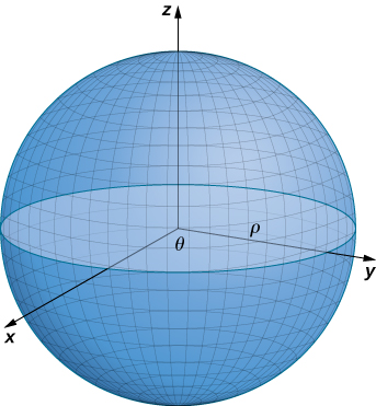
We have discussed parameterizations of various surfaces, but two important types of surfaces need a separate discussion: spheres and graphs of two-variable functions. To parameterize a sphere, it is easiest to use spherical coordinates. The sphere of radius \(\rho\) centered at the origin is given by the parameterization
\(\mathbf r(\phi,\theta) = \langle \rho \, \cos \theta \, \sin \phi, \, \rho \, \sin \theta \, \sin \phi, \, \rho \, \cos \phi \rangle, \, 0 \leq \theta \leq 2\pi, \, 0 \leq \phi \leq \pi.\)
The idea of this parameterization is that as \(\phi\) sweeps downward from the positive \(z\)-axis, a circle of radius \(\rho \, \sin \phi\) is traced out by letting \(\theta\) run from 0 to \(2\pi\). To see this, let \(\phi\) be fixed. Then
\[\begin{align*} x^2 + y^2 &= (\rho \, \cos \theta \, \sin \phi)^2 + (\rho \, \sin \theta \, \sin \phi)^2 \\[4pt]
&= \rho^2 \sin^2 \phi (\cos^2 \theta + \sin^2 \theta) \\[4pt]
&= \rho^2 \, \sin^2 \phi \\[4pt]
&= (\rho \, \sin \phi)^2. \end{align*}\]
This results in the desired circle (Figure \(\PageIndex{5}\)).
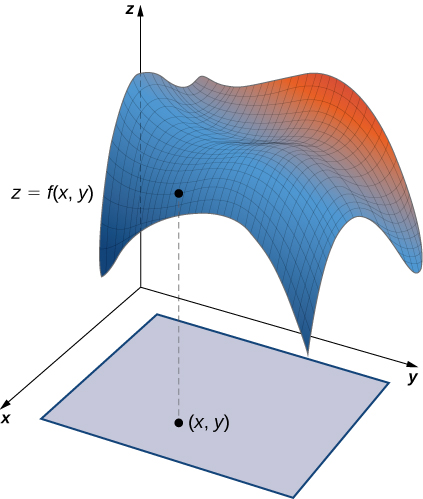
Finally, to parameterize the graph of a two-variable function, we first let \(z = f(x,y)\) be a function of two variables. The simplest parameterization of the graph of \(f\) is \(\mathbf r(x,y) = \langle x,y,f(x,y) \rangle\), where \(x\) and \(y\) vary over the domain of \(f\) (Figure \(\PageIndex{6}\)). For example, the graph of \(f(x,y) = x^2 y\) can be parameterized by \(\mathbf r(x,y) = \langle x,y,x^2y \rangle\), where the parameters \(x\) and \(y\) vary over the domain of \(f\). If we only care about a piece of the graph of \(f\) - say, the piece of the graph over rectangle \([ 1,3] \times [2,5]\) - then we can restrict the parameter domain to give this piece of the surface:
\[\mathbf r(x,y) = \langle x,y,x^2y \rangle, \, 1 \leq x \leq 3, \, 2 \leq y \leq 5.\]
Similarly, if \(S\) is a surface given by equation \(x = g(y,z)\) or equation \(y = h(x,z)\), then a parameterization of \(S\) is \(\mathbf r(y,z) = \langle g(y,z), \, y,z\rangle\) or \(\mathbf r(x,z) = \langle x,h(x,z), z\rangle\), respectively. For example, the graph of paraboloid \(2y = x^2 + z^2\) can be parameterized by \(\mathbf r(x,y) = \left\langle x, \dfrac{x^2+z^2}{2}, z \right\rangle, \, 0 \leq x < \infty, \, 0 \leq z < \infty\). Notice that we do not need to vary over the entire domain of \(y\) because \(x\) and \(z\) are squared.
Let’s now generalize the notions of smoothness and regularity to a parametric surface. Recall that curve parameterization \(\mathbf r(t), \, a \leq t \leq b\) is regular (or smooth) if \(\mathbf r'(t) \neq \mathbf 0\) for all \(t\) in \([a,b]\). For a curve, this condition ensures that the image of \(\mathbf r\) really is a curve, and not just a point. For example, consider curve parameterization \(\mathbf r(t) = \langle 1,2\rangle, \, 0 \leq t \leq 5\). The image of this parameterization is simply point \((1,2)\), which is not a curve. Notice also that \(\mathbf r'(t) = \mathbf 0\). The fact that the derivative is the zero vector indicates we are not actually looking at a curve.
Analogously, we would like a notion of regularity (or smoothness) for surfaces so that a surface parameterization really does trace out a surface. To motivate the definition of regularity of a surface parameterization, consider the parameterization
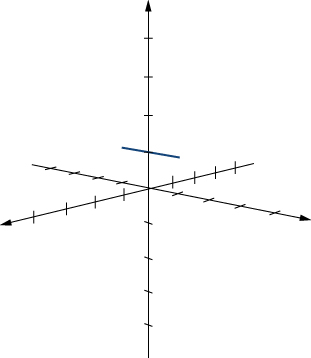
\[\mathbf r(u,v) = \langle 0, \, \cos v, \, 1 \rangle, \, 0 \leq u \leq 1, \, 0 \leq v \leq \pi.\]
Although this parameterization appears to be the parameterization of a surface, notice that the image is actually a line (Figure \(\PageIndex{7}\)). How could we avoid parameterizations such as this? Parameterizations that do not give an actual surface? Notice that \(\mathbf r_u = \langle 0,0,0 \rangle\) and \(\mathbf r_v = \langle 0, -\sin v, 0\rangle\), and the corresponding cross product is zero. The analog of the condition \(\mathbf r'(t) = \mathbf 0\) is that \(\mathbf r_u \times \mathbf r_v\) is not zero for point \((u,v)\) in the parameter domain, which is a regular parameterization.
Parameterization \(\mathbf r(u,v) = \langle x(u,v), y(u,v), z(u,v) \rangle\) is a regular parameterization if \(\mathbf r_u \times \mathbf r_v\) is not zero for point \((u,v)\) in the parameter domain.
If parameterization \(\vec{r}\) is regular, then the image of \(\vec{r}\) is a two-dimensional object, as a surface should be. Throughout this chapter, parameterizations \(\mathbf r(u,v) = \langle x(u,v), y(u,v), z(u,v) \rangle\)are assumed to be regular.
Recall that curve parameterization \(\mathbf r(t), \, a \leq t \leq b\) is smooth if \(\mathbf r'(t)\) is continuous and \(\mathbf r'(t) \neq \mathbf 0\) for all \(t\) in \([a,b]\). Informally, a curve parameterization is smooth if the resulting curve has no sharp corners. The definition of a smooth surface parameterization is similar. Informally, a surface parameterization is smooth if the resulting surface has no sharp corners.
A surface parameterization \(\mathbf r(u,v) = \langle x(u,v), y(u,v), z(u,v) \rangle\) is smooth if vector \(\mathbf r_u \times \mathbf r_v\) is not zero for any choice of \(u\) and \(v\) in the parameter domain.
Is the surface parameterization \(\mathbf r(u,v) = \langle u^{2v}, v + 1, \, \sin u \rangle, \, 0 \leq u \leq 2, \, 0 \leq v \leq 3\) smooth?
- Hint
-
Investigate the cross product \(\mathbf r_u \times \mathbf r_v\).
- Answer
-
Yes
Surface Area of a Parametric Surface
Our goal is to define a surface integral, and as a first step we have examined how to parameterize a surface. The second step is to define the surface area of a parametric surface. The notation needed to develop this definition is used throughout the rest of this chapter.
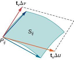
Let \(S\) be a surface with parameterization \(\mathbf r(u,v) = \langle x(u,v), \, y(u,v), \, z(u,v) \rangle\) over some parameter domain \(D\). We assume here and throughout that the surface parameterization \(\mathbf r(u,v) = \langle x(u,v), \, y(u,v), \, z(u,v) \rangle\) is continuously differentiable—meaning, each component function has continuous partial derivatives. Assume for the sake of simplicity that \(D\) is a rectangle (although the following material can be extended to handle nonrectangular parameter domains). Divide rectangle \(D\) into subrectangles \(D_{ij}\) with horizontal width \(\Delta u\) and vertical length \(\Delta v\). Suppose that i ranges from 1 to m and j ranges from 1 to n so that \(D\) is subdivided into mn rectangles. This division of \(D\) into subrectangles gives a corresponding division of surface \(S\) into pieces \(S_{ij}\). Choose point \(P_{ij}\) in each piece \(S_{ij}\). Point \(P_{ij}\) corresponds to point \((u_i, v_j)\) in the parameter domain.
Note that we can form a grid with lines that are parallel to the \(u\)-axis and the \(v\)-axis in the \(uv\)-plane. These grid lines correspond to a set of grid curves on surface \(S\) that is parameterized by \(\mathbf r(u,v)\). Without loss of generality, we assume that \(P_{ij}\) is located at the corner of two grid curves, as in Figure \(\PageIndex{9}\). If we think of \(\mathbf r\) as a mapping from the \(uv\)-plane to \(\mathbb{R}^3\), the grid curves are the image of the grid lines under \(\mathbf r\). To be precise, consider the grid lines that go through point \((u_i, v_j)\). One line is given by \(x = u_i, \, y = v\); the other is given by \(x = u, \, y = v_j\). In the first grid line, the horizontal component is held constant, yielding a vertical line through \((u_i, v_j)\). In the second grid line, the vertical component is held constant, yielding a horizontal line through \((u_i, v_j)\). The corresponding grid curves are \(\mathbf r(u_i, v)\) and \((u, v_j)\) and these curves intersect at point \(P_{ij}\).
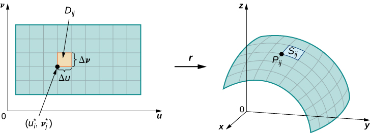
Now consider the vectors that are tangent to these grid curves. For grid curve \(\mathbf r(u_i,v)\), the tangent vector at \(P_{ij}\) is
\[\mathbf t_v (P_{ij}) = \mathbf r_v (u_i,v_j) = \langle x_v (u_i,v_j), \, y_v(u_i,v_j), \, z_v (u_i,v_j) \rangle.\]
For grid curve \(\mathbf r(u, v_j)\), the tangent vector at \(P_{ij}\) is
\[\mathbf t_u (P_{ij}) = \mathbf r_u (u_i,v_j) = \langle x_u (u_i,v_j), \, y_u(u_i,v_j), \, z_u (u_i,v_j) \rangle.\]
If vector \(\mathbf N = \mathbf t_u (P_{ij}) \times \mathbf t_v (P_{ij})\) exists and is not zero, then the tangent plane at \(P_{ij}\) exists (Figure \(\PageIndex{10}\)). If piece \(S_{ij}\) is small enough, then the tangent plane at point \(P_{ij}\) is a good approximation of piece \(S_{ij}\).
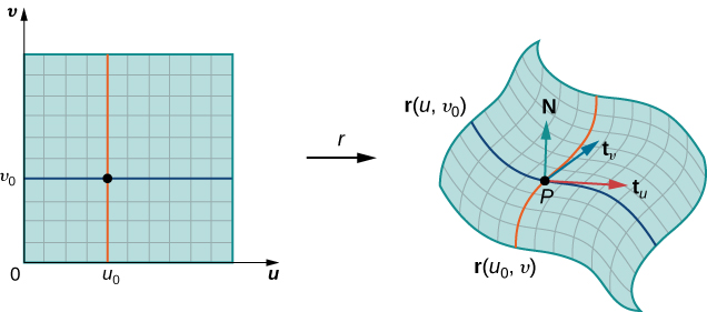
The tangent plane at \(P_{ij}\) contains vectors \(\mathbf t_u(P_{ij})\) and \(\mathbf t_v(P_{ij})\) and therefore the parallelogram spanned by \(\mathbf t_u(P_{ij})\) and \(\mathbf t_v(P_{ij})\) is in the tangent plane. Since the original rectangle in the \(uv\)-plane corresponding to \(S_{ij}\) has width \(\Delta u\) and length \(\Delta v\), the parallelogram that we use to approximate \(S_{ij}\) is the parallelogram spanned by \(\Delta u \mathbf t_u(P_{ij})\) and \(\Delta v \mathbf t_v(P_{ij})\). In other words, we scale the tangent vectors by the constants \(\Delta u\) and \(\Delta v\) to match the scale of the original division of rectangles in the parameter domain. Therefore, the area of the parallelogram used to approximate the area of \(S_{ij}\) is
\[\Delta S_{ij} \approx ||(\Delta u \mathbf t_u (P_{ij})) \times (\Delta v \mathbf t_v (P_{ij})) || = ||\mathbf t_u (P_{ij}) \times \mathbf t_v (P_{ij}) || \Delta u \,\Delta v.\]
Varying point \(P_{ij}\) over all pieces \(S_{ij}\) and the previous approximation leads to the following definition of surface area of a parametric surface (Figure \(\PageIndex{11}\)).
Let \(\mathbf r(u,v) = \langle x(u,v), \, y(u,v), \, z(u,v) \rangle\) with parameter domain \(D\) be a smooth parameterization of surface \(S\). Furthermore, assume that \(S\) is traced out only once as \((u,v)\) varies over \(D\). The surface area of \(S\) is
\[\iint_D ||\mathbf t_u \times \mathbf t_v || \,dA, \label{equation1}\]
where \(\mathbf t_u = \left\langle \dfrac{\partial x}{\partial u},\, \dfrac{\partial y}{\partial u},\, \dfrac{\partial z}{\partial u} \right\rangle\)
and
\[\mathbf t_v = \left\langle \dfrac{\partial x}{\partial v},\, \dfrac{\partial y}{\partial v},\, \dfrac{\partial z}{\partial v} \right\rangle.\]
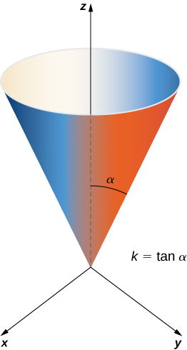
Calculate the lateral surface area (the area of the “side,” not including the base) of the right circular cone with height h and radius r.
Solution
Before calculating the surface area of this cone using Equation \ref{equation1}, we need a parameterization. We assume this cone is in \(\mathbb{R}^3\) with its vertex at the origin (Figure \(\PageIndex{12}\)). To obtain a parameterization, let \(\alpha\) be the angle that is swept out by starting at the positive z-axis and ending at the cone, and let \(k = \tan \alpha\). For a height value \(v\) with \(0 \leq v \leq h\), the radius of the circle formed by intersecting the cone with plane \(z = v\) is \(kv\). Therefore, a parameterization of this cone is
\[\mathbf s(u,v) = \langle kv \, \cos u, \, kv \, \sin u, \, v \rangle, \, 0 \leq u < 2\pi, \, 0 \leq v \leq h. \nonumber\]
The idea behind this parameterization is that for a fixed \(v\)-value, the circle swept out by letting \(u\) vary is the circle at height \(v\) and radius \(kv\). As \(v\) increases, the parameterization sweeps out a “stack” of circles, resulting in the desired cone.
With a parameterization in hand, we can calculate the surface area of the cone using Equation \ref{equation1}. The tangent vectors are \(\mathbf t_u = \langle - kv \, \sin u, \, kv \, \cos u, \, 0 \rangle\) and \(\mathbf t_v = \langle k \, \cos u, \, k \, \sin u, \, 1 \rangle\). Therefore,
\begin{align*} \vecs t_u \times \vecs t_v &= \begin{vmatrix} \mathbf{\hat{i}} & \mathbf{\hat{j}} & \mathbf{\hat{k}} \\ -kv \sin u & kv \cos u & 0 \\ k \cos u & k \sin u & 1 \end{vmatrix} \\[4pt] &= \langle kv \, \cos u, \, kv \, \sin u, \, -k^2 v \, \sin^2 u - k^2 v \, \cos^2 u \rangle \\[4pt] &= \langle kv \, \cos u, \, kv \, \sin u, \, - k^2 v \rangle. \end{align*}
The magnitude of this vector is
\[ \begin{align*} ||\langle kv \, \cos u, \, kv \, \sin u, \, -k^2 v \rangle || &= \sqrt{k^2 v^2 \cos^2 u + k^2 v^2 \sin^2 u + k^4v^2} \\[4pt] &= \sqrt{k^2v^2 + k^4v^2} \\[4pt] &= kv\sqrt{1 + k^2}. \end{align*}\]
By Equation \ref{equation1}, the surface area of the cone is
\[ \begin{align*}\iint_D ||\mathbf t_u \times \mathbf t_v|| \, dA &= \int_0^h \int_0^{2\pi} kv \sqrt{1 + k^2} \,du\, dv \\[4pt] &= 2\pi k \sqrt{1 + k^2} \int_0^h v \,dv \\[4pt] &= 2 \pi k \sqrt{1 + k^2} \left[\dfrac{v^2}{2}\right]_0^h \\[4pt] \\[4pt] &= \pi k h^2 \sqrt{1 + k^2}. \end{align*}\]
Since \(k = \tan \alpha = r/h\),
\[ \begin{align*} \pi k h^2 \sqrt{1 + k^2} &= \pi \dfrac{r}{h}h^2 \sqrt{1 + \dfrac{r^2}{h^2}} \\[4pt] &= \pi r h \sqrt{1 + \dfrac{r^2}{h^2}} \\[4pt] \\[4pt] &= \pi r \sqrt{h^2 + h^2 \left(\dfrac{r^2}{h^2}\right) } \\[4pt] &= \pi r \sqrt{h^2 + r^2}. \end{align*}\]
Therefore, the lateral surface area of the cone is \(\pi r \sqrt{h^2 + r^2}\).
AnalysisThe surface area of a right circular cone with radius \(r\) and height \(h\) is usually given as \(\pi r^2 + \pi r \sqrt{h^2 + r^2}\). The reason for this is that the circular base is included as part of the cone, and therefore the area of the base \(\pi r^2\) is added to the lateral surface area \(\pi r \sqrt{h^2 + r^2}\) that we found.
Find the surface area of the surface with parameterization \(\mathbf r(u,v) = \langle u + v, \, u^2, \, 2v \rangle, \, 0 \leq u \leq 3, \, 0 \leq v \leq 2\).
- Hint
-
Use Equation \ref{equation1}.
- Answer
-
\(\≈ 43.02\)
Show that the surface area of the sphere \(x^2 + y^2 + z^2 = r^2\) is \(4 \pi r^2\).
Solution
The sphere has parameterization
\(r \, \cos \theta \, \sin \phi, \, r \, \sin \theta \, \sin \phi, \, r \, \cos \phi \rangle, \, 0 \leq \theta < 2\pi, \, 0 \leq \phi \leq \pi.\)
The tangent vectors are
\(\mathbf t_{\theta} = \langle -r \, \sin \theta \, \sin \phi, \, r \, \cos \theta \, \sin \phi, \, 0 \rangle\)
and
\(\mathbf t_{\phi} = \langle r \, \cos \theta \, \cos \phi, \, r \, \sin \theta \, \cos \phi, \, -r \, \sin \phi \rangle.\)
Therefore,
\[ \begin{align*}\mathbf t_{\phi} \times \mathbf t_{\theta} &= \langle r^2 \cos \theta \, \sin^2 \phi, \, r^2 \sin \theta \, \sin^2 \phi, \, r^2 \sin^2 \theta \, \sin \phi \, \cos \phi + r^2 \cos^2 \theta \, \sin \phi \, \cos \phi \rangle \\[4pt] &= \langle r^2 \cos \theta \, \sin^2 \phi, \, r^2 \sin \theta \, \sin^2 \phi, \, r^2 \sin \phi \, \cos \phi \rangle. \end{align*}\]
Now,
\[ \begin{align*}||\mathbf t_{\phi} \times \mathbf t_{\theta} || &= \sqrt{r^4\sin^4\phi \, \cos^2 \theta + r^4 \sin^4 \phi \, \sin^2 \theta + r^4 \sin^2 \phi \, \cos^2 \phi} \\[4pt] &= \sqrt{r^4 \sin^4 \phi + r^4 \sin^2 \phi \, \cos^2 \phi} \\[4pt] &= r^2 \sqrt{\sin^2 \phi} \\[4pt] &= r \, \sin \phi.\end{align*}\]
Notice that \(\sin \phi \geq 0\) on the parameter domain because \(0 \leq \phi < \pi\), and this justifies equation \(\sqrt{\sin^2 \phi} = \sin \phi\). The surface area of the sphere is
\[\int_0^{2\pi} \int_0^{\pi} r^2 \sin \phi \, d\phi \,d\theta = r^2 \int_0^{2\pi} 2 \, d\theta = 4\pi r^2. \nonumber\]
We have derived the familiar formula for the surface area of a sphere using surface integrals.
Show that the surface area of cylinder \(x^2 + y^2 = r^2, \, 0 \leq z \leq h\) is \(2\pi rh\). Notice that this cylinder does not include the top and bottom circles.
- Hint
-
Use the standard parameterization of a cylinder and follow the previous example.
- Answer
-
With the standard parameterization of a cylinder, Equation \ref{equation1} shows that the surface area is \(2 \pi rh\).
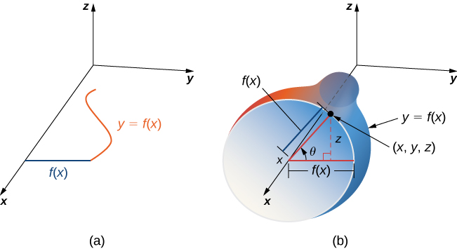
In addition to parameterizing surfaces given by equations or standard geometric shapes such as cones and spheres, we can also parameterize surfaces of revolution. Therefore, we can calculate the surface area of a surface of revolution by using the same techniques. Let \(y = f(x) \geq 0\) be a positive single-variable function on the domain \(a \leq x \leq b\) and let \(S\) be the surface obtained by rotating \(f\) about the \(x\)-axis (Figure \(\PageIndex{13}\)). Let \(\theta\) be the angle of rotation. Then, \(S\) can be parameterized with parameters \(x\) and \(\theta\) by
\[\mathbf r(x, \theta) = \langle x, f(x) \, \cos \theta, \, f(x) \sin \theta \rangle, \, a \leq x \leq b, \, 0 \leq x \leq 2\pi.\]
Find the area of the surface of revolution obtained by rotating \(y = x^2, \, 0 \leq x \leq b\) about the x-axis (Figure \(\PageIndex{14}\)).
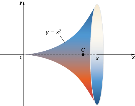
Solution
This surface has parameterization \(\mathbf r(x, \theta) = \langle x, \, x^2 \cos \theta, \, x^2 \sin \theta \rangle, \, 0 \leq x \leq b, \, 0 \leq x < 2\pi.\)
The tangent vectors are \( \mathbf t_x = \langle 1, \, 2x \, \cos \theta, \, 2x \, \sin \theta \rangle\) and \(\mathbf t_{\theta} = \langle 0, \, -x^2 \sin \theta, \, -x^2 \cos \theta \rangle\).
Therefore,
\[\begin{align*} \mathbf t_x \times \mathbf t_{\theta} &= \langle 2x^3 \cos^2 \theta + 2x^3 \sin^2 \theta, \, -x^2 \cos \theta, \, -x^2 \sin \theta \rangle \\[4pt] &= \langle 2x^3, \, -x^2 \cos \theta, \, -x^2 \sin \theta \rangle \end{align*}\]
and
\[\begin{align*} \mathbf t_x \times \mathbf t_{\theta} &= \sqrt{4x^6 + x^4\cos^2 \theta + x^4 \sin^2 \theta} \\[4pt] &= \sqrt{4x^6 + x^4} \\[4pt] &= x^2 \sqrt{4x^2 + 1} \end{align*}\]
The area of the surface of revolution is
\[\begin{align*} \int_0^b \int_0^{2\pi} x^2 \sqrt{4x^2 + 1} \, d\theta \,dx &= 2\pi \int_0^b x^2 \sqrt{4x^2 + 1} \,dx \\[4pt]
&= 2\pi \left[ \dfrac{1}{64} \left(2 \sqrt{4x^2 + 1} (8x^3 + x) \, \sinh^{-1} (2x)\right)\right]_0^b \\[4pt]
&= 2\pi \left[ \dfrac{1}{64} \left(2 \sqrt{4b^2 + 1} (8b^3 + b) \, \sinh^{-1} (2b) \right)\right]. \end{align*}\]
Use Equation \ref{equation1} to find the area of the surface of revolution obtained by rotating curve \(y = \sin x, \, 0 \leq x \leq \pi\) about the \(x\)-axis.
- Hint
-
Use the parameterization of surfaces of revolution given before Example \(\PageIndex{7}\).
- Answer
-
\(2\pi (\sqrt{2} + \sinh^{-1} (1))\)
Key Concepts
- Surfaces can be parameterized, just as curves can be parameterized. In general, surfaces must be parameterized with two parameters.
- Surfaces can sometimes be oriented, just as curves can be oriented.
- If \(S\) is a surface, then the area of \(S\) is \[\iint_S \, dS.\]
Glossary
- Grid curves
- curves on a surface that are parallel to grid lines in a coordinate plane
- Parameter domain (parameter space)
- the region of the \(uv\)-plane over which the parameters \(u\) and \(v\) vary for parameterization \(\mathbf r(u,v) = \langle x(u,v), \, y(u,v), \, z(u,v)\rangle\)
- Parameterized surface (parametric surface)
- a surface given by a description of the form \(\mathbf r(u,v) = \langle x(u,v), \, y(u,v), \, z(u,v)\rangle\), where the parameters \(u\) and \(v\) vary over a parameter domain in the \(uv\)-plane
- Regular parameterization
- parameterization \(\mathbf r(u,v) = \langle x(u,v), \, y(u,v), \, z(u,v)\rangle\) such that \(r_u \times r_v\) is not zero for point \((u,v)\) in the parameter domain
- Surface area
- the area of surface \(S\) given by the surface integral \[\iint_S \,dS\]
Contributors and Attributions
Gilbert Strang (MIT) and Edwin “Jed” Herman (Harvey Mudd) with many contributing authors. This content by OpenStax is licensed with a CC-BY-SA-NC 4.0 license. Download for free at http://cnx.org.
It follows from Example \(\PageIndex{1}\) that we can parameterize all cylinders of the form \(x^2 + y^2 = R^2\). If S is a cylinder given by equation \(x^2 + y^2 = R^2\), then a parameterization of \(S\) is \(\mathbf r(u,v) = \langle R \, \cos u, \, R \, \sin u, \, v \rangle, \, 0 \leq u \leq 2 \pi, \, -\infty < v < \infty.\)
We can also find different types of surfaces given their parameterization, or we can find a parameterization when we are given a surface.
Example \(\PageIndex{2}\): Describing a Surface
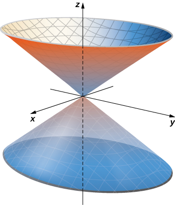
Describe surface \(S\) parameterized by \(\mathbf r(u,v) = \langle u \, \cos v, \, u \, \sin v, \, u^2 \rangle, \, 0 \leq u < \infty, \, 0 \leq v < 2\pi\).
Solution
Notice that if \(u\) is held constant, then the resulting curve is a circle of radius \(u\) in plane \(z = u\). Therefore, as \(u\) increases, the radius of the resulting circle increases. If \(v\) is held constant, then the resulting curve is a vertical parabola. Therefore, we expect the surface to be an elliptic paraboloid. To confirm this, notice that
\[\begin{align*} x^2 + y^2 &= (u \, \cos v)^2 + (u \, \sin v)^2 \\[4pt] &= u^2 \cos^2 v + u^2 sin^2 v \\[4pt] &= u^2 \\[4pt] &=z\end{align*}\]
Therefore, the surface is the elliptic paraboloid \(x^2 + y^2 = z\) (Figure \(\PageIndex{3}\)).
Exercise \(\PageIndex{2}\)
Describe the surface parameterized by \(\mathbf r(u,v) = \langle u \, \cos v, \, u \, \sin v, \, u \rangle, \, - \infty < u < \infty, \, 0 \leq v < 2\pi\).
Hold \(u\) constant and see what kind of curves result. Imagine what happens as \(u\) increases or decreases.
Cone \(x^2 + y^2 = z^2\)