3.5: Maxima and Minima

Let us assume throughout this section that \(f\) is a real function whose domain is an interval \(I\), and furthermore that \(f\) is continuous on \(I\). A problem that often arises is that of finding the point \(c\) where \(f(c)\) has its largest value, and also the point \(c\) where \(f(c)\) has its smallest value. The derivative turns out to be very useful in this problem. We begin by defining the concepts of maximum and minimum.

Definition:

Let \(c\) be a real number in the domain \(I\) of \(f\).
(i)  \(f\) has a maximum at \(c\) if \(f(c) \geq f(x)\) for all real numbers \(x\) in \(I\). In this case \(f(c)\) is called the maximum value of \(f\).
(ii) \(f\) has a minimum at \(c\) if \(f(c) \leq f(x)\) for all real numbers \(x\) in \(I\). \(f(c)\) is then called the minimum value of \(f\).

When we look at the graph of a continuous function \(f\) on \(I\), the maximum will appear as the highest peak and the minimum as the lowest valley (Figure \(\PageIndex{1}\)).

Figure \(\PageIndex{1}\): Maximum and minimum.

In general, all of the following possibilities can arise:

\(f\) has no maximum in its domain \(I\).
\(f\) has a maximum at exactly one point in \(I\).
\(f\) has a maximum at several different points in \(I\).

However even if \(f\) has a maximum at several different points, \(f\) can have only one maximum value. Because if \(f\) has a maximum at \(c_{1}\) and also at \(c_{2}\), then \(f\left(c_{1}\right) \geq f\left(c_{2}\right)\) and \(f\left(c_{2}\right) \geq f\left(c_{1}\right)\), and therefore \(f\left(c_{1}\right)\) and \(f\left(c_{2}\right)\) are equal.

Example \(\PageIndex{1}\)

Each of the following functions, graphed in Figure \(\PageIndex{2}\), have no maximum and no minimum:

a) \(f(x) = 1/x, \quad 0 < x\)
b) \(f(x) = x^{2}, \quad 0 < x < 1\)
c) \(f(x) = 2x + 3\)

Figure \(\PageIndex{2}\): No maximum or minimum.

Example \(\PageIndex{2}\)

The function \(f(x) = x^{2} + 1\) has no maximum. But \(f\) has a minimum at \(x = 0\) with value \(1\), because for \(x \neq 0\), we always have \(x^{2} > 0\), \(x^{2} + 1 > 1\). The graph is shown in Figure \(\PageIndex{2}\).

Figure \(\PageIndex{3}\): Graph of \(f(x) = x^{2} + 1\).

The use of the derivative in finding maxima and minima is based on the Critical Point Theorem. It shows that the maxima and minima of a function can only occur at certain points, called critical points. The theorem will be stated now, and its proof is given at the end of this section.

Critical Point Theorem

Let \(f\) have domain \(I\). Suppose that \(c\) is a point in \(I\) and \(I\) has either a maximum or a minimum at \(c\). Then one of the following three things must happen:

\(\begin{align*} &&(\text{i}) \ &c \text{ is an endpoint of } I, \\ &&(\text{ii}) \ &f'(c) \text{ is undefined}, \\ &&(\text{iii}) \ &f'(c) = 0. \end{align*}\)

We shall say that \(c\) is a critical point of \(f\) if either (i), (ii), or (iii) happens. The three types of critical points are shown in Figure \(\PageIndex{4}\). When \(I\) is an open interval, (i) cannot arise since the endpoints are not elements of \(I\). But when \(I\) is a closed interval, the two endpoints of \(I\) will always be among the critical points. Geometrically the theorem says that if \(f\) has a maximum or minimum at \(c\), then either \(c\) is an endpoint of the curve, or there is a sharp corner at \(c\), or the curve has a horizontal slope at \(c\). Thus at a maximum there is either an endpoint, a sharp peak, or a horizontal summit.

Figure \(\PageIndex{4}\): Critical Point Theorem.

The Critical Point Theorem has some important applications to economics. Here is one example. Some other examples are described in the problem set.

Example \(\PageIndex{3}\)

Suppose a quantity \(x\) of a commodity can be produced at a total cost \(C(x)\) and sold for a total revenue of \(R(x)\), \(0 < x < \infty\). The profit is defined as the difference between the revenue and the cost, \[P(x) = R(x) - C(x). \nonumber\]

Show that if the profit has a maximum at \(x_{0}\), then the marginal cost is equal to the marginal revenue at \(x_{0}\), \[R' \left(x_{0}\right) = C' \left(x_{0}\right). \nonumber\]

In this problem it is understood that \(R(x)\) and \(C(x)\) are differentiable functions, so that the marginal cost and marginal revenue always exist. Therefore \(P'(x)\) exists and \[P'(x) = R'(x) - C'(x). \nonumber\]

Assume \(P(x)\) has a maximum at \(x_{0}\). Since \((0, \infty)\) has no endpoints and \(P'\left(x_{0}\right)\) exists, the Critical Point Theorem shows that \(P'\left(x_{0}\right) = 0\). Thus \[P'\left(x_{0}\right) = R'\left(x_{0}\right) - C'\left(x_{0}\right) = 0 \nonumber\]

and \[R'\left(x_{0}\right) = C'\left(x_{0}\right). \nonumber\]

Definition:

An interior point of an interval \(I\) is an element of \(I\) which is not an endpoint of \(I\).

For example, if \(I\) is an open interval, then every point of \(I\) is an interior point of \(I\). But if \(I\) is a closed interval \([a, b]\), then the set of all interior points of \(I\) is the open interval \((a, b)\) (Figure \(\PageIndex{5}\)).

Figure \(\PageIndex{5}\): Endpoints and interior points.

An interior point of I which is a critical point off is called an interior critical point. There are a number of tests to determine whether or not \(f\) has a maximum at a given interior critical point. Here are two such tests. In both tests we assume that \(f\) is continuous on its domain \(I\).

Direct Test

Suppose \(c\) is the only interior critical point of \(f\), and \(u\), \(v\) are points in \(I\) with \(u < c < v\).

\(\begin{align*} &&(\text{i}) \ &\text{If } f(c) > f(u) \text{ and } f(c) > f(v), \text{ then } f \text{ has a maximum at } c \text{ and nowhere else.} \\ &&(\text{ii}) \ &\text{If } f(c) < f(u) \text{ and } f(c) < f(v), \text{ then } f \text{ has a minimum at } c \text{ and nowhere else.} \\ &&(\text{iii}) \ &\text{Otherwise, } f \text{ has neither a maximum nor a minimum at } c. \end{align*}\)

The three cases in the Direct Test are shown in Figure \(\PageIndex{6}\). The advantage of the Direct Test is that one can determine whether \(f\) has a maximum or minimum at \(c\) by computing only the three values \(f(u)\), \(f(v)\), and \(f(c)\) instead of computing all values of \(f(x)\).

Figure \(\PageIndex{6}\): The cases possible for the Direct Test.

Proof of the Direct Test

We must prove that if two points of \(I\) are on the same side of \(c\), their values are on the same side of \(f(c)\). Suppose, for instance, that \(u_{1} < u_{2} < c\) (Figure \(\PageIndex{7}\)). On the close interval \([u_{1}, c]\) the only critical points are the endpoints. Thus when we restrict \(f\) to this interval, it has a maximum at one endpoint and a minimum at the other. If the maximum is at \(c\), then \(f(u_{1})\) and \(f(u_{2})\) are both less than \(f(c)\); if the minimum is at \(c\), then \(f(u_{1})\) and \(f(u_{2})\) are both greater than \(f(c)\). A similar proof works when \(c < v_{1} < v_{2}\).

Figure \(\PageIndex{7}\): Cases possible for the Direct Test.

Note: our proof used the fact that \(f\) has a maximum and a minimum on each closed interval. That fact, called the Extreme Value Theorem, will be proved in Section 3.8.

Second Derivative Test

Suppose \(c\) is the only interior critical point of \(f\) and that \(f'(c) = 0\).

\(\begin{align*} &&(\text{i}) \ &\text{If } f''(c) < 0, f \text{ has a maximum at } c \text{ and nowhere else.} \\ &&(\text{ii}) \ &\text{If } f''(c) > 0, f \text{ has a minimum at } c \text{ and nowhere else.} \end{align*}\)

We omit the proof and give a simple intuitive argument instead. (See Figure \(\PageIndex{8}\).) Since \(f'(c) = 0\), the curve is horizontal at \(c\). If \(f''(c)\) is negative the slope is decreasing. This means that the curve climbs up until it levels off at \(c\) and then falls down, so it has a maximum at \(c\). On the other hand, if \(f"(c)\) is positive, the slope is increasing, so the curve falls down until it reaches a minimum at \(c\) and then climbs up. This argument makes it easy to remember which way the inequalities go in the test.

Figure \(\PageIndex{8}\): Cases possible for the Second Derivative Test.

The Second Derivative Test fails when \(f''(c) = 0\) and when \(f''(c)\) does not exist. When the Second Derivative Test fails any of the following things can still happen:

1. \(f\) has a maximum at \(x = c\).
2. \(f\) has a minimum at \(x = c\).
3. \(f\) has neither a maximum nor a minimum at \(x = c\).

In most maximum and minimum problems, there is only one critical point except for the endpoints of the interval. We develop a method for finding the maximum and minimum in that case.

Method for Finding Maxima and Minima

When to use: \(f\) is continuous on its domain \(I\), and \(f\) has exactly one interior critical point.

Step 1: Differentiate \(f\).
Step 2: Find the unique interior critical point \(c\) of \(f\).
Step 3: Test to see whether \(f\) has a maximum or minimum at \(c\). The Direct Test or the Second Derivative Test may be used.

This method can be applied to an open or half-open interval as well as a closed interval. The Second Derivative Test is more convenient because it requires only the single computation \(f''(c)\), while the Direct Test requires the three computations \(f(u)\), \(f(v)\), and \(f(c)\). However, the Direct Test always works while the Second Derivative Test sometimes fails.

We illustrate the use of both tests in the examples.

Example \(\PageIndex{4}\)

Find the point on the line \(y = 2x + 3\) which is at minimum distance from the origin.

Solution

The distance is given by \[z = \sqrt{x^{2} + y^{2}}, \nonumber\]and substituting \(2x + 3\) for \(y\), \[z = \sqrt{x^{2} + (2x + 3)^{2}} = \sqrt{5x^{2} + 12x + 9}. \nonumber\]

This is defined on the whole real line. 

Step 1: \(\dfrac{dz}{dx} = \dfrac{10x + 12}{2 \sqrt{5x^{2} + 12x + 9}} = \dfrac{5x + 6}{z}.\)

Step 2: \(\dfrac{dz}{dx} = 0\) only when \(5x + 6 = 0\), or \(x = - \dfrac{6}{5}\).

Step 3: \(\dfrac{d^{2}z}{dx^{2}} = \dfrac{5z - (5x + 6)(dz/dx)}{z^{2}}\).

At \(x = -\frac{6}{5}\), \(5x + 6 = 0\) and \(z > 0\) so \(d^{2}z/dx^{2} = 5/z > 0\). By the Second Derivative Test, \(z\) has a minimum at \(x = -\frac{6}{5}\).

Conclusion

The distance is a minimum at \(x = -\frac{6}{5}\), \(y = 2x + 3 = \frac{3}{5}\). The minimum distance is \(z = \sqrt{x^{2} + y^{2}} = \sqrt{\frac{9}{5}}\). This is shown in Figure \(\PageIndex{9}\).

Figure \(\PageIndex{9}\). Graph of \(y = 2x + 3\) with its point of minimum distance from the origin indicated. 

Example \(\PageIndex{5}\)

Find the minimum of \(f(x) = x^{6} + 10x^{4} + 2\).

Solution

Step 1: \(f'(x) = 6x^{5} + 40x^{3} = x^{3} \left(6x^{2} + 40\right)\).

Step 2: \(f'(x) = 0\) only when \(x = 0\).

Step 3: The Second Derivative Test fails, because \[f''(x) = 30x^{4} + 120x^{2}, \quad f''(0) = 0. \nonumber\]We use the Direct Test. Let \(u = -1\), \(v = 1\). Then \[f(0) = 2, \quad f(-1) = 13, \quad f(1) = 13. \nonumber\]Hence \(f\) has a minimum at 0, as shown in Figure \(\PageIndex{10}\).

Figure \(\PageIndex{10}\): Graph of \(f(x) = x^{6} + 10x^{4} + 2\) with the function minimum indicated.

Example \(\PageIndex{6}\)

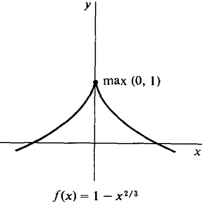
Find the maximum of \(f(x) = 1 - x^{2/3}\).

Solution

Step 1: \(f'(x) = - \left(\frac{2}{3}\right) x^{-1/3}\).

Step 2: \(f'(x)\) is undefined at \(x = 0\), and this is the only critical point.

Step 3: We use the Direct Test. Let \(u = -1\), \(v = 1\). \[f(0) = 1, \quad f( -1) = 0, \quad f(I) = 0. \nonumber\]Thus \(f\) has a maximum at \(x = 0\), as shown in Figure \(\PageIndex{11}\).

Figure \(\PageIndex{11}\): Graph of \(f(x) = 1 - x^{2/3}\) with the function maximum indicated.

If \(f\) has more than one interior critical point, the maxima and minima can sometimes be found by dividing the interval into two or more parts.

Example \(\PageIndex{7}\)

Find the maximum and minimum of \(f(x) = x/\left(x^{2} + 1\right)\).

Solution

Step 1: \(f'(x) = \dfrac{(x^{2} + 1) - 2x^{2}}{(x^{2} + 1)^{2}} = \dfrac{1 - x^{2}}{(x^{2} + 1)^{2}}\).

Step 2: \(f'(x) = 0\) when \(x = -1\) and \(x = 1\). There are two interior critical points. We divide the interval \((-\infty, \infty)\) on which \(f\) is defined into the two subintervals \((-\infty, 0]\) and \([0, \infty)\). On each of these subintervals, \(f\) has just one interior critical point.

Step 3: We shall use the direct test for the subinterval \((-\infty, 0]\). At the critical point \(-1\), we have \(f(-1) = -1\). By direct computation, we see that
\(f(-2) = -\frac{2}{5}\) and \(f(0) = 0\). Both of these values are greater than \(-1\). This shows that the restriction of \(f\) to the subinterval \((-\infty, 0]\) has a minimum at \(x = -1\). Moreover, \(f(x)\) is always \(\geq 0\) for \(x\) in the other subinterval \([0, \infty)\). Therefore \(f\) has a minimum at \(-1\) for the whole interval \((-\infty, \infty)\). In a similar way, we can show that \(f\) has a maximum at \(x = 1\).

Conclusion
\(f\) has a minimum at \(x = -1\) with value \(f(-1) = -\frac{1}{2}\), and a maximum at \(x = 1\) with value \(f(1) = 1\). (See Figure \(\PageIndex{12}\).)

Figure \(\PageIndex{12}\): Graph of \(f(x) = \frac{x}{1 + x^{2}}\) with the function maximum and minimum indicated.

The Critical Point Theorem can often be used to show that a curve has no maximum or minimum on an open interval \(I = (a, b)\). The theorem shows that:

If \(y = f(x)\) has no critical points in \((a, b)\), the curve has no maximum or minimum on \((a, b)\).
If \(y = f(x)\) has just one critical point \(x = c\) in \((a, b)\) and two points \(x_{1}\) and \(x_{2}\) are found where \(f(x_{1}) < f(c) < f(x_{2})\), then the curve has no maximum or minimum on \((a, b)\).

Example \(\PageIndex{8}\)

\(f(x) = x^{3} - 1\). Test for maxima and minima.

Solution

Step 1: \(f'(x) = 3x^{2}\).

Step 2: \(f'(x) = 0\) only when \(x = 0\).

Step 3: The Second Derivative Test fails, because \(f''(x) = 6x, \quad \(f''(0) = 0\). By direct computation, \(f(0) = -1, \quad f(-1) = 2, \quad f(1) = 0\). Therefore \(f\) has neither a minimum nor a maximum at \(x = 0\).

Conclusion
Since \(x = 0\) is the only critical point of \(f\) and \(f\) doesn't have a maximum or minimum there, we conclude that \(f\) has no maximum and no minimum as shown in Figure \(\PageIndex{13}\).

Figure \(\PageIndex{13}\): Graph of \(x^{3} - 1\) with magnified view of the region around its critical point \((0, -1)\).

Proof of the Critical Point Theorem

Assume that neither \((\text{i})\) nor \((\text{ii})\) of the Critical Point Theorem holds; that is, assume that \(c\) is not an endpoint of \(I\) and \(f'(c)\) exists. We must show that \((\text{iii})\) is true; i.e., \(f'(c) = 0\). We give the proof for the case that \(f\) has a maximum at \(c\). Let \(x = c\), and let \(\Delta x > 0\) be infinitesimal. Then \[f(c + \Delta x) \leq f(c), \quad f(c - \Delta x) \leq f(c). \nonumber\]

(See \(\PageIndex{14}\). Therefore \[\frac{f(c + \Delta x) - f(c)}{\Delta x} \leq 0 \leq \frac{f(c - \Delta x) - f(c)}{-\Delta x}. \nonumber\]

Figure \(\PageIndex{14}\): Proof of the Critical Point Theorem.

Taking standard parts, \[f'(c) = st \left(\frac{f(c + \Delta x) - f(c)}{\Delta x}\right) \leq 0, \nonumber\]and also, \[0 \leq st \left(\frac{f(c - \Delta x) - f(c)}{\Delta x}\right) = f'(c). \nonumber\]

Therefore \(f'(0) = c\).

Problems for Section 3.5.5

In Problems 1-36, find the unique interior critical point and determine whether it is a maximum, a minimum, or neither.

1.	\(f(x) = x^{2}\)	2.	\(f(x) = 1 - x^{2}\)
3.	\(f(x) = x^{4} + 2\)	4.	\(f(x) = x^{4} + 3x^{2} + 5\)
5.	\(f(x) = x^{3} + 2\)	6.	\(f(x) = x^{3} - 3x^{2} + 3x\)
7.	\(f(x) = 3x^{2} + 2x - 5\)	8.	\(f(x) = 2(x-1)^{4} + (x-1)^{2} + 6\)
9.	\(f(x) = x^{4/5}\)	10.	\(f(x) = 2 - (x+1)^{2/3}\)
11.	\(f(x) = \dfrac{1}{x^{2} - 1}, \quad -1 < x < 1\)	12.	\(f(x) = \dfrac{1}{x^{2} + 1}\)
13.	\(f(x) = x^{1/3} + 1\)	14.	\(f(x) = 4 - x^{1/5}\)
15.	\(f(x) = x^{2} - x^{-1}, \quad x < 0\)	16.	\(f(x) = x^{2} - x^{-1}, \quad x > 0\)
17.	\(f(x) = x^{-1} - (x - 3)^{-1}, \quad 0 < x < 3\)	18.	\(f(x) = x + x^{-1}, \quad 0 < x\)
19.	\(f(x) = \sqrt{4 - x^{2}}, \quad -2 \leq x \leq 2\)	20.	\(f(x) = \left(4 - x^{2}\right)^{-1/2}, \quad -2 < x < 2\)
21.	\(y = \sin x + x, \quad 0 \leq x \leq 2\pi\)	22.	\(y = \sin^{2} x, \quad 0 < x < \pi\)
23.	\(y = e^{-x^{2}}\)	24.	\(y = e^{x^{2} - 1}\)
25.	\(y = \dfrac{1}{\cos x}, \quad -\dfrac{\pi}{2} < x < \dfrac{\pi}{2}\)	26.	\(y = \ln (\sin x), \quad 0 < x < \pi\)
27.	\(y = xe^{x}\)	28.	\(y = x \ln x, \quad 0 < x < \infty\)
29.	\(y = x - \ln x, \quad 0 < x < \infty\)	30.	\(y = e^{x} - x\)
31.	\(f(x) = |x - 3|\)	32.	\(f(x) = 3 + |1 - x|\)
33.	\(f(x) = 2 - |x|\)	34.	\(f(x) = 2|x| - x\)
35.	\(f(x) = \sqrt{x} + \sqrt{1 - x}, \quad 0 \leq x \leq 1\)	36.	\(f(x) = \sqrt{x} + \sqrt{9 - 3x}, \quad 0 \leq x \leq 3\)
37.	Find the shortest distance between the line \(y = 1 - 4x\) and the origin.
38.	Find the shortest distance between the curve \(y = 2/x\) and the origin.
39.	Find the minimum of the curve \(f(x) = x^{m} - mx, x > 0\), where \(m\) is an integer \(\geq 2\).
40.	Find the minimum of the curve \(f(x) = x^{m} - mx, x < 0\), where \(m\) is an odd integer \(\geq 2\).

In Problems 41-44, find the maximum and minimum of the given curve.

41.	\(f(x) = \dfrac{x}{x^{2} + 4}\)	42.	\(f(x) = \dfrac{3x + 4}{x^{2} + 1}\)
43.	\(f(x) = \dfrac{x}{x^{4} + 1}\)	44.	\(f(x) = \dfrac{x^{3}}{x^{4} + 1}\)