3.4: Continuity

Intuitively, a curve $y = f(x)$ is continuous if it forms an unbroken line, that is, whenever $x_{1}$ is close to $x_{2}$, $f\left(x_{1}\right)$ is close to $f\left(x_{2}\right)$. To make this intuitive idea into a mathematical definition, we substitute “infinitely close” for “close”.

Definition:

$f$ is said to be continuous at a point $c$ if:

$\begin{align*} &(\text{i}) \ && f \text{ is defined at } c; \\ &(\text{ii}) && \text{whenever } x \text{ is infinitely close to } c, f(x) \text{ is infinitely close to } f(c). \end{align*}$

If $f$ is not continuous at $c$ it is said to be discontinuous at $c$.

When $f$ is continuous at $c$, the entire part of the curve where $x \approx c$ will be visible in an infinitesimal microscope aimed at the point $(c, f(c))$, as shown in Figure $\PageIndex{1(\text{a})}$. But if $f$ is discontinuous at $c$, some values of $f(x)$ where $x \approx c$ will either be undefined or outside the range of vision of the microscope, as in Figure $\PageIndex{1(\text{b})}$.

Continuity, like the derivative, can be expressed in terms of limits. Again the proof is immediate from the definitions.

Figure $\PageIndex{1}$: Continuous and discontinuous functions.

Theorem $\PageIndex{1}$

$f$ is continuous at $c$ if and only if $$\lim_{x \rightarrow c} f(x) = f(c). \nonumber$$

As an application, we have a set of rules for combining continuous functions. They can be proved either by the corresponding rules for limits (Table $\PageIndex{1}$ in Section 3.3) or by computing standard parts.

Theorem $\PageIndex{2}$

Suppose $f$ and $g$ are continuous at $c$.

$\begin{align*} &(\text{i}) \ &&\text{For any constant } k, \text{ the function } k \cdot f(x) \text{ is continuous at } c. \\ &(\text{ii}) \ &&f(x) + g(x) \text{ is continuous at } c. \\ &(\text{iii}) \ &&f(x) \cdot g(x) \text{ is continuous at } c. \\ &(\text{iv}) \ &&\text{If } g(c) \neq 0, \text{then } f(x) / g(x) \text{ is continuous at } c. \\ &(\text{v}) \ && \text{If } f(c) \text{ is positive and } n \text{is an integer, then } \sqrt[n]{f(x)} \text{ is continuous at } c. \end{align*}$

By repeated use of Theorem $\PageIndex{2}$, we see that all of the following functions are continuous at $c$.

• Every polynomial function.
• Every rational function $f(x) / g(x)$, where $f(x)$ and $g(x)$ are polynomials and $g(c) \neq 0$.
• The functions $f(x) = x^{r}$, where $r$ is rational and $x$ is positive.

Sometimes a function $f(x)$ will be undefined at a point $x = c$ while the limit $$L = \lim_{x \rightarrow c} f(x). \nonumber$$ exists. When this happens, we can make the function continuous at $c$ by defining $f(c) = L$.

Example $\PageIndex{1}$

Let $f(x) = \dfrac{x^{2} + x - 2}{x - 1}$.

At any point $c \neq 1$ $f$ is continuous. But $f(1)$ is undefined so $f$ is discontinuous at 1. However, $$\lim_{x \rightarrow 1} \frac{x^{2} + x - 2}{x - 1} = \lim_{x \rightarrow 1} \frac{(x - 1)(x + 2)}{x - 1} = 3. \nonumber$$

We can make $f$ continuous at $1$ by defining $$f(x) = \begin{cases} \frac{x^{2} + x - 2}{x - 1} \quad &\text{if } x \neq 1, \\ 3 &\text{if } x = 1. \end{cases} \nonumber$$

(See Figure $\PageIndex{2}$.)

Figure $\PageIndex{2}$: Defining a piecewise function that avoids discontinuity. 

In terms of a dependent variable $y = f(x)$, the definition of continuity takes the following form, where $\Delta y = f(c + \Delta x) - f(c)$.

Definition:

$y$ is continuous at $x = c$ if: 

$\begin{align*} &(\text{i}) \ &&y \text{ is defined at } c. \\ &(\text{ii}) \ &&\text{Whenever } \Delta x \text{ is infinitesimal, } \Delta y \text{ is infinitesimal}. \end{align*}$

To summarize, given a function $y = f(x)$ defined at $x = c$, all the statements below are equivalent.

1. $f$ is continuous at $c$.
2. Whenever $x \approx c$, $f(x) \approx f(c)$.
3. Whenever $st(x) = c$, $st(f(x)) = f(c)$.
4. $\displaystyle \lim_{x \rightarrow c} f(x) = f(c)$.
5. $y$ is continuous at $x = c$.
6. Whenever $\Delta x$ is infinitesimal, $\Delta y$ is infinitesimal.

Our next theorem is that differentiability implies continuity. That is, the set of differentiable functions at $c$ is a subset of the set of continuous functions at $c$. (See Figure $\PageIndex{3}$.)

Figure $\PageIndex{3}$.

Theorem $\PageIndex{3}$

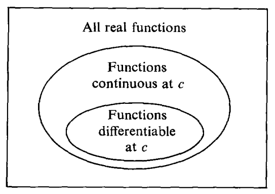
If $f$ is differentiable at $c$ then $f$ is continuous at $c$.

Proof

Let $y = f(x)$, and let $\Delta x$ be a nonzero infinitesimal. Then $\Delta y/\Delta x$ is infinitely close to $f'(c)$ and is therefore finite. Thus $\Delta y = \Delta x(\Delta y/\Delta x)$ is the product of an infinitesimal and a finite number, so $\Delta y$ is infinitesimal.

For example, the transcendental functions $\sin x$, $\cos x$, $e^{x}$ are continuous for all $x$, and $\ln x$ is continuous for $x > 0$. Theorem $\PageIndex{3}$ can be used to show that combinations of these functions are continuous.

Example $\PageIndex{2}$

Find as large a set as you can on which the function $$f(x) = \frac{\sin x \ln (x + 1)}{x^{2} - 4} \nonumber$$ is continuous.

Solution

$\sin x$ is continuous for all $x$. $\ln (x + 1)$ is continuous whenever $x + 1 > 0$, that is, $x > - 1$. The numerator $\sin x \ln (x + 1)$ is thus continuous whenever $x > -1$. The denominator $x^{2} - 4$ is continuous for all $x$ but is zero when $x = \pm 2$. Therefore $f(x)$ is continuous whenever $x > -1$ and $x \neq 2$.

The next two examples give functions which are continuous but not differentiable at a point $c$.

Example $\PageIndex{3}$

The function $y = x^{1/3}$ is continuous but not differentiable at $x = 0$. (See Figure \(\PageIndex{4 \text{(a)}\).) We have seen before that it is not differentiable at $x = 0$. It is continuous because if $\Delta x$ is infinitesimal then so is $$\Delta y = (0 + \Delta x)^{1/3} - 0^{1/3} = (\Delta x)^{1/3}. \nonumber$$

Example $\PageIndex{4}$

The absolute value function $y = |x|$ is continuous but not differentiable at the point $x = 0$. (See Figure \(\PageIndex{4 \text{(b)}\).) 

We have already shown that the derivative does not exist at $x = 0$. To see that the function is continuous, we note that for any infinitesimal $\Delta x$, $$\Delta y = |0 + \Delta x| - |0| = \Delta x. \nonumber$$ and thus $\Delta y$ is infinitesimal.

Figure $\PageIndex{4}$: Graphs of (a) $y = x^{1/3}$ and (b) $y = |x|$.

The path of a bouncing ball is a series of parabolas shown in Figure $\PageIndex{5}$. The curve is continuous everywhere. At the points $a_{1}, a_{2}, a_{3}, \ldots$ where the ball bounces, the curve is continuous but not differentiable. At other points, the curve is both continuous and differentiable.

Figure $\PageIndex{5}$: Path of bouncing ball.

In the classical kinetic theory of gases, a gas molecule is assumed to be moving at a constant velocity in a straight line except at the instant of time when it collides with another molecule or the wall of the container. Its path is then a broken line in space, as in Figure $\PageIndex{6}$.

Figure $\PageIndex{6}$: Path of an ideal gas molecule.

The position in three dimensional space at time $t$ can be represented by three functions $$x= f(t), \quad y = g(t), \quad z = h(t). \nonumber$$

All three functions, $f$, $g$, and $h$ are continuous for all values of $t$. At the time $t$ of a collision, at least one and usually all three derivatives $dx/dt$, $dy/dt$,(dz/dt\) will be undefined because the speed or direction of the molecule changes abruptly. At any other time $t$, when no collision is taking place, all three derivatives $dx/dt$, $dy/dt$, $dz/dt$ will exist.

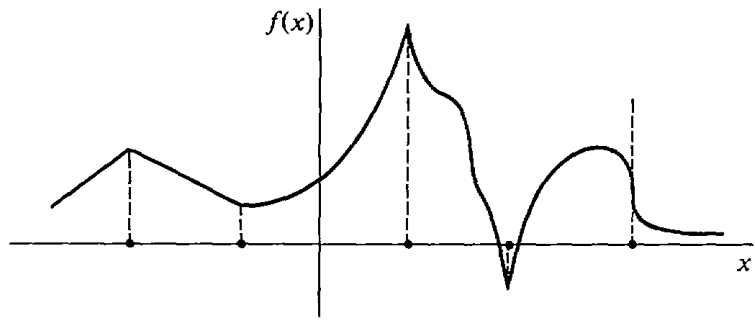
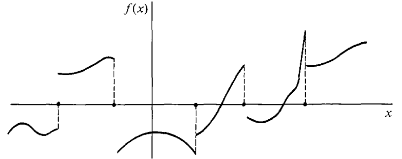
The functions we shall ordinarily encounter in this book will be defined and have a derivative at all but perhaps a finite number of points of an interval. The graph of such a function will be a smooth curve where the derivative exists. At points where the curve has a sharp corner (like $0$ in $|x|$) or a vertical tangent line (like $0$ in $x^{1/3}$), the function is continuous but not differentiable (see Figure $\PageIndex{7}$). At points where the function is undefined or there is a jump, or the value approaches infinity or oscillates wildly, the function is discontinuous (see Figure $\PageIndex{8}$).

Figure $\PageIndex{7}$: Points where $f$ is continuous but nondifferentiable.

Figure $\PageIndex{8}$: Points where $f$ is discontinuous.

The next theorem is similar to the Chain Rule for derivatives.

Theorem $\PageIndex{4}$

If $f$ is continuous at $c$ and $G$ is continuous at $f(c)$, then the function $$g(x) = G(j(x)) \nonumber$$ is also continuous at $c$. That is, a continuous function of a continuous function is continuous.

Proof

Let $x$ be infinitely close to but not equal to $c$. Then $$st(g(x)) = st(G(j(x))) = G(st(f(x))) = G(j(c)) = g(c). \nonumber$$ For example, the following functions are continuous: $$\begin{align*} f(x) &= \sqrt{x^{2} + 1} \quad &&\text{all } x \\ g(x) &= \left|x^{3} - x\right| &&\text{all } x \\ h(x) &= \left(1 + \sqrt{x}\right)^{1/3} &&x > 0 \\ j(x) &= e^{\sin x} && \text{all } x \\ k(x) &= \ln |x| &&\text{all } x \neq 0 \end{align*}$$

Here are two examples illustrating two types of discontinuities.

Example $\PageIndex{5}$

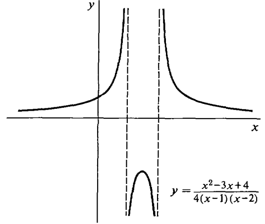
The function $g(x) = \dfrac{x^{2} - 3x + 4}{4(x-1)(x-2)}$ is continuous at every real point except $x = 1$ and $x = 2$. At these two points
$g(x)$ is undefined (Figure $\PageIndex{9}$).

Figure $\PageIndex{9}$: Graph of $y = \dfrac{x^{2} - 3x + 4}{4(x-1)(x-2)}$.

Example $\PageIndex{6}$

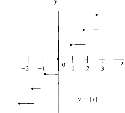
The greatest integer function $[x]$, shown in Figure $\PageIndex{10}$, is defined by $$[x] = \text{the greatest integer } n \text{ such that } n \leq x. \nonumber$$ Thus $[x] = 0$ if $0 \leq x < 1$, $[x] = 1$ if $1 \leq x < 2$, $[x] = 2$ if $2 \leq x < 3$, and so on. For negative $x$, we have $[x] = -1$ if $-1 \leq x < 0$, $[x] = -2$ if $-2 \leq x < -1$, and so on. For example, if $-2 \leq x < -1$, and so on. For example, $$[7.362] = 7, \quad [\pi] = 3, \quad [-2.43] = -3. \nonumber$$

For each integer $n$, $[n]$ is equal to $n$. The function $[x]$ is continuous when $x$ is not an integer but is discontinuous when $x$ is an integer $n$. At an integer $n$, both one-sided limits exist but are different, $$\lim_{x \rightarrow n^{-}} f(x) = n - 1, \quad \lim_{x \rightarrow n^{+}} f(x) = n. \nonumber$$

The graph of $[x]$ looks like a staircase. It has a step, or jump discontinuity, at each integer $n$. The function $[x]$ will be useful in the last section of this chapter. Some hand calculators have a key for either the greatest integer function or for the similar function that gives $[x]$ for positive $x$ and $[x] + 1$ for negative $x$.

Figure $\PageIndex{10}$: Graph of the greatest integer function, $y = [x]$.

Functions which are "continuous on an interval" will play an important role in this chapter. Intervals were discussed in Section 1.1. Recall that closed intervals have the form
$$[a, b], \nonumber$$

open intervals have one of the forms $$(a, b), \quad (a, \infty), \quad (-\infty, b), \quad (-\infty, \infty), \nonumber$$ and half-open intervals have one of the forms $$[a, b), \quad (a, b], \quad [a, \infty), \quad (-\infty, b]. \nonumber$$ In these intervals, $a$ is called the lower endpoint and $b$, the upper endpoint. The symbol $-\infty$ indicates that there is no lower endpoint, while $\infty$ indicates that there is no upper endpoint.

Definition:

We say that $f$ is continuous on an open interval $I$ if $f$ is continuous at every point $c$ in $I$. If in addition $f$ has a derivative at every point of $I$, we say that $f$ is differentiable on $I$.

To define what is meant by a function continuous on a closed interval, we introduce the notions of continuous from the right and continuous from the left, using one-sided limits.

Definition:

$f$ is continuous from the right at $c$ if $\displaystyle \lim_{x \rightarrow c^{+}} f(x) = f(c).$

$f$ is continuous from the left at $c$ if $\displaystyle \lim_{x \rightarrow c^{-}} f(x) = f(c).$

Example $\PageIndex{6}$ (continued)

The greatest integer function $f(x) = [x]$ is continuous from the right but not from the left at each integer $n$ because $$[n] = n, \quad \lim_{x \rightarrow n^{+}} [x] = n, \quad \lim_{x \rightarrow n^{-}} [x] = n - 1. \nonumber$$

It is easy to check that $f$ is continuous at $c$ if and only if $f$ is continuous from both the right and left at $c$.

Definition:

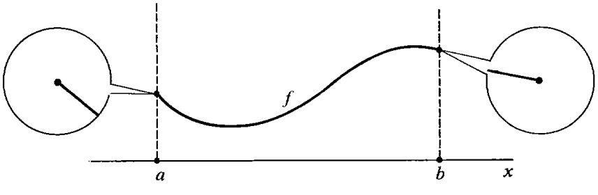
$f$ is said to be continuous on the closed interval $[a, b]$ if $f$ is continuous at each point $c$ where $a < c < b$, continuous from the right at $a$, and continuous from the left at $b$.

Figure $\PageIndex{11}$ shows a function $f$ continuous on $[a, b]$.

Figure $\PageIndex{11}$: $f$ is continuous on the interval $[a, b]$.

Example $\PageIndex{7}$

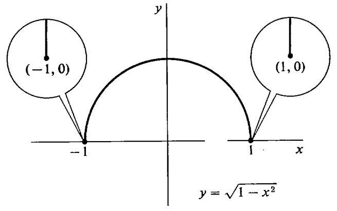
The semicircle $$y = \sqrt{1 - x^{2}} \nonumber$$ shown in Figure $\PageIndex{12}$ is continuous on the closed interval $[-1, 1]$. It is differentiable on the open interval $(-1, 1)$. To see that it is continuous from the right at $x = -1$, let $\Delta x$ be positive infinitesimal. Then $$\begin{align*} y &= \sqrt{1 - (-1)^{2}} = 0 \\ y + \Delta y &= \sqrt{1 - (-1 + \Delta x)^{2}} = \sqrt{1 - (1 - 2\Delta x + (\Delta x)^{2})} \\ &= \sqrt{2 \Delta x - (\Delta x)^{2}} = \sqrt{(2 - \Delta x)\Delta x}. \end{align*}$$

Thus $$y = \sqrt{(2 - \Delta x) \Delta x}. \nonumber$$ The number inside the radical is positive infinitesimal, so $\Delta y$ is infinitesimal. This shows that the function is continuous from the right at $x = - 1$. Similar reasoning shows it is continuous from the left at $x = 1$.

Figure $\PageIndex{12}$: Graph of $y = \sqrt{1 - x^{2}}$.

Problems for Section 3.4

In Problems 1-17, find the set of all points at which the function is continuous.

1.	$f(x) = 3x^{2} + 5x + 4$	2.	$f(x) = \dfrac{5x + 2}{x^{2} + 1}$
3.	$f(x) = \sqrt{x + 2}$	4.	$f(x) = \dfrac{x}{x + 2}$
5.	$f(x) = \sqrt{|x - 2| + 1}$	6.	$f(x) = \dfrac{x + 3}{|x + 3|}$
7.	$f(x) = \dfrac{x}{x^{2} + x}$	8.	$f(x) = \dfrac{x + 2}{(x - 1)(x - 3)^{1/3}}$
9.	$f(x) = \sqrt{4 - x^{2}}$	10.	$f(x) = \sqrt{x^{2} - 4}$
11.	$f(x) = \dfrac{1}{x - (1/(x + 1))}$	12.	$g(x) = \dfrac{1}{x} + \dfrac{1}{x - 1}$
13.	$g(x) = \dfrac{x - 2}{x - 3} + \dfrac{x - 3}{x - 2}$	14.	$g(x) = \sqrt{x^{3} - x}$
15.	$g(x) = \sqrt[4]{x^{2} - x^{3}}$	16.	$f(t) = \sqrt{t^{-2} - 1}$
17.	$f(x) = \sqrt{t^{-1} - 1}$
18.	Show that $f(x) = \sqrt{x}$ is continuous from the right at $x = 0$.
19.	Show that $f(x) = \sqrt{1 - x}$ is continuous from the left at $x = 1$.
20.	Show that $f(x) = \sqrt{1 - |x|}$ is continuous on the closed interval $[- 1, 1]$.
21.	Show that $f(x) = \sqrt{x} + \sqrt{2 - x}$ is continuous on the closed interval $[0, 2]$.
22.	Show that $f(x) = \sqrt{9 - x^{2}}$ is continuous on the closed interval $[-3, 3]$.
23.	Show that $f(x) = \sqrt{x^{2} - 9}$ is continuous on the half-open intervals $(-\infty, - 3]$ and $[3, \infty)$).
$\square$ 24.	Suppose the function $f(x)$ is continuous on the closed interval $[a, b]$. Show that there is a function $g(x)$ which is continuous on the whole real line and has the value $g(x) = f(x)$ for $x$ in $[a, b]$.
$\square$ 25.	Suppose $\displaystyle \lim_{x \rightarrow c} f(x) = L$. Prove that the function $g(x)$, defined by $g(x) = f(x)$ for $x \neq c$ and $g(x) = L$ for $x = c$, is continuous at $c$.
26.	In the curve $y = f(x)$ illustrated below, identify the points $x = c$ where each of the following happens: (a) $f$ is discontinuous at $x = c$ (b) $f$ is continuous but not differentiable at $x = c$.