4.1: The Definite Integral

We shall begin our study ofthe integral calculus in the same way in which we began with the differential calculus—by asking a question about curves in the plane.

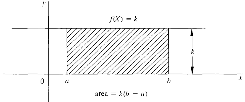
Suppose $f$ is a real function continuous on an interval $I$ and consider the curve $y = f(x)$. Let $a < b$ where $a$, $b$ are two points in $I$, and let the curve be above the $x$-axis for $x$ between $a$ and $b$; that is, $f(x) \geq 0$. We then ask: What is meant by the area of the region bounded by the curve $y = f(x)$, the $x$-axis, and the lines $x = a$ and $x = b$? That is, what is meant by the area of the shaded region in Figure $\PageIndex{1}$? We call this region the region under the curve $y = f(x)$ between $a$ and $b$.

Figure $\PageIndex{1}$: The region under a curve.

The simplest possible case is where $f$ is a constant function; that is, the curve is a horizontal line $f(x) = k$, where $k$ is a constant and $k \neq 0$, shown in Figure(\PageIndex{2}\). In this case the region under the curve is just a rectangle with height $k$ and width $b - a$, so the area is defined as $$\text{Area} = k \cdot (b - a). \nonumber$$ The areas of certain other simple regions, such as triangles, trapezoids, and semicircles, are given by formulas from plane geometry.

Figure $\PageIndex{2}$: Area of a region under a constant function.

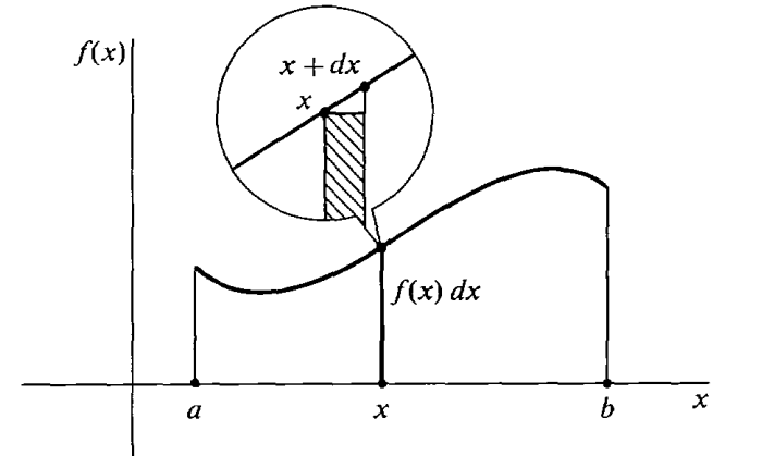
The area under any continuous curve $y = f(x)$ will be given by the definite integral, which is written $$\int_{a}^{b} f(x) \ dx. \nonumber$$ Before plunging into the detailed definition of the integral, we outline the main ideas.

First, the region under the curve is divided into infinitely many vertical strips of infinitesimal width $dx$. Next, each vertical strip is replaced by a vertical rectangle of height $f (x)$, base $dx$, and area $f(x) \ dx$. The next step is to form the sum of the areas of all these rectangles, called the infinite Riemann sum (look ahead to Figures $\PageIndex{3}$ and $\PageIndex{11}$). Finally, the integral $\int_{a}^{b} f(x) \ dx$ is defined as the standard part of the infinite Riemann sum.

The infinite Riemann sum, being a sum of rectangles, has an infinitesimal error. This error is removed by taking the standard part to form the integral. 

It is often difficult to compute an infinite Riemann sum, since it is a sum of infinitely many infinitesimal rectangles. We shall first study finite Riemann sums, which can easily be computed on a hand calculator.

Suppose we slice the region under the curve between $a$ and $b$ into thin vertical strips of equal width. If there are $n$ slices, each slice will have width $\Delta x = (b - a)/n$. The interval $[a, b]$ will be partitioned into $n$ subintervals $$\left[x_{0}, x_{1}\right], \ \left[x_{1}, x_{2}\right], \ \ldots, \ \left[x_{n - 1}, x_{n}\right] \nonumber$$ where $x_{0} = a, \ x_{1} = a + \Delta x, \ x_{2} = a + 2\Delta x, \ \ldots, \ x_{n} = b.$

The points $x_{0}, \ x_{1}, \ \ldots, \ x_{n}$ are called partition points. On each subinterval $\left[x_{k-1}, x_{k}\right]$, we form the rectangle of height $f\left(x_{k-1}\right)$. The $k$^th rectangle will have area $$f\left(x_{k-1}\right) \cdot \Delta x. \nonumber$$

From Figure $\PageIndex{3}$, we can see that the sum of the areas of all these rectangles will be fairly close to the area under the curve. This sum is called a Riemann sum and is equal to $$f\left(x_{0}\right) \Delta x + f\left(x_{1}\right) \Delta x + \cdots + f\left(x_{n-1}\right) \Delta x. \nonumber$$

It is the area of the shaded region in the picture. A convenient way of writing Riemann sums is the $\sum$-notation" ($\sum$ is the capital Greek letter sigma), $$\sum_{a}^{b} f(x) \ \Delta x = f\left(x_{0}\right) \Delta x + f\left(x_{1}\right) \Delta x + \cdots + f\left(x_{n-1}\right) \Delta x. \nonumber$$ The $a$ and $b$ indicate that the first subinterval begins at $a$ and the last subinterval ends at $b$.

Figure $\PageIndex{3}$: The Riemann Sum.

We can carry out the same process even when the subinterval length $\Delta x$ does not divide evenly into the interval length $b - a$. But then, as Figure $\PageIndex{4}$ shows, there will be a remainder left over at the end of the interval $[a, b]$, and the Riemann sum will have an extra rectangle whose width is this remainder. We let $n$ be the largest integer such that $$a + n\Delta x \leq b, \nonumber$$ and we consider the subintervals $$\left[x_{0}, x_{1}\right], \ \ldots, \ \left[x_{n-1}, x_{n}\right], \ \left[x_{n}, b\right], \nonumber$$ where the partition points are $$x_{0} = a, \ x_{1} = a + \Delta x, \ x_{2} = a + 2\Delta x, \ \ldots, \ x_{n} = a + n \Delta x, \ b. \nonumber$$

Figure $\PageIndex{1}$: Riemann Sum where interval does not evenly divide into subintervals.

$x_{n}$ will be less than or equal to $b$ but $x_{n} + \Delta x$ will be greater than $b$. Then we define the Riemann sum to be the sum $$\sum_{a}^{b} f(x) \ \Delta x = f \left(x_{0}\right) \ \Delta x + f \left(x_{1}\right) \ \Delta x + \cdots + f \left(x_{n-1}\right) \ \Delta x + f \left(x_{n}\right) \left(b - x_{n}\right). \nonumber$$

Thus given the function $f$, the interval $[a, \ b]$, and the real number $\Delta x > 0$, we have defined the Riemann sum $\sum_{a}^{b} f(x) \ \Delta x$. We repeat the definition more concisely.

Definition: Term

Let $a < b$ and let $\Delta x$ be a posltlve real number. Then the Riemann sum $\sum_{a}^{b} f(x) \ \Delta x$ is defined as the sum  $$\sum_{a}^{b} f(x) \ \Delta x = f \left(x_{0}\right) \ \Delta x + f \left(x_{1}\right) \ \Delta x + \cdots + f \left(x_{n-1}\right) \ \Delta x + f \left(x_{n}\right) \left(b - x_{n}\right) \nonumber$$

where $n$ is the largest integer such that $a + n \Delta x \leq b$, and  $$x_{0} = a, \ x_{1} = a + \Delta x, \ x_{2} = a + 2\Delta x, \ \ldots, \ x_{n} = a + n \Delta x, \ b \nonumber$$ are the partition points.

If $x_{0} = b$, the last term $f \left(x_{n}\right) \left(b - x_{n}\right)$ is zero. The Riemann sum $\sum_{a}^{b} f(x) \ \Delta x$ is a real function of three variables $a$, $b$, and $\Delta x$, $$\sum_{a}^{b} f(x) \ \Delta x = S(a, b, \Delta x). \nonumber$$ The symbol $x$ which appears in the expression is called a dummy variable (or bound variable), because the value of $\sum_{a}^{b} f(x) \ \Delta x$ does not depend on $x$. The dummy variable allows us to use more compact notation, writing $f(x) \ \Delta x$ just once instead of writing $f \left(x_{0}\right) \Delta x$, $f \left(x_{1}\right) \Delta x$, $f \left(x_{2}\right) \Delta x$, and so on.

From Figure $\PageIndex{5}$ it is plausible that by making $\Delta x$ smaller we can get the Riemann sum as close to the area as we wish.

Figure $\PageIndex{5}$: Accuracy of approximation by Riemann sum varies based on the number of partitions.

Example $\PageIndex{1}$

Let $f(x) = \frac{1}{2}x$. In Figure $\PageIndex{6}$, the region under the curve from $x = 0$ to $x = 2$ is a triangle with base 2 and height 1, so its area should be $$A = \frac{1}{2} bh = 1. \nonumber$$

Figure $\PageIndex{6}$: Exact area of $f(x) = \frac{1}{2} x$ on $[0, 2]$.

Let us compare this value for the area with some Riemann sums. In Figure $\PageIndex{7}$, we take $\Delta x = \frac{1}{2}$. The interval $[0, 2]$ divides into four subintervals $[0, \frac{1}{2}]$, $[\frac{1}{2}, 1]$, $[1, \frac{3}{2}]$ and $[\frac{3}{2}, 2]$. We make a table of values of $f(x)$ at the lower endpoints.

$x_{k}$	$0$	$\frac{1}{2}$	$1$	$\frac{3}{2}$
$f \left(x_{k}\right)$	$0$	$\frac{1}{4}$	$\frac{1}{2}$	$\frac{3}{4}$

Figure $\PageIndex{7}$: Riemann sum with 4 equal subintervals and function values measured at lower endpoints.

The Riemann sum is then $$\sum_{0}^{2} f(x) \ \Delta x = 0 \cdot \frac{1}{2} + \frac{1}{4} \cdot \frac{1}{2} + \frac{1}{2} \cdot \frac{1}{2} + \frac{3}{4} \cdot \frac{1}{2} = \frac{6}{8}. \nonumber$$

In Figure $\PageIndex{8}$, we take $\Delta x = \frac{1}{4}$. The table of values is as follows.

$x_{k}$	$0$	$\frac{1}{4}$	$\frac{2}{4}$	$\frac{3}{4}$	$\frac{4}{4}$	$\frac{5}{4}$	$\frac{6}{4}$	$\frac{7}{4}$
$f \left(x_{k}\right)$	$0$	$\frac{1}{8}$	$\frac{2}{8}$	$\frac{3}{8}$	$\frac{4}{8}$	$\frac{5}{8}$	$\frac{6}{8}$	$\frac{7}{8}$

The Riemann sum is $$\sum_{0}^{2} f(x) \ \Delta x = 0 \cdot \frac{1}{4} + \frac{1}{8} \cdot \frac{1}{4} + \frac{2}{8} \cdot \frac{1}{4} + \frac{3}{8} \cdot \frac{1}{4} + \frac{4}{8} \cdot \frac{1}{4} + \frac{5}{8} \cdot \frac{1}{4} + \frac{6}{8} \cdot \frac{1}{4} + \frac{7}{8} \cdot \frac{1}{4} = \frac{7}{8} \nonumber$$ We see that the value is getting closer to one.

Figure $\PageIndex{8}$: Riemann sum with 8 equal subintervals and function values measured at lower endpoints.

Finally, let us take a value of $\Delta x$ that does not divide evenly into the interval length 2. Let $\Delta x= 0.6$. We see in Figure $\PageIndex{9}$ that the interval then divides into three subintervals of length 0.6 and one of length 0.2, namely $[0, 0.6]$, $[0.6, 1.2]$, $[1.2, 1.8]$, $[1.8, 2.0]$.

$x_{k}$	$0$	$0.6$	$1.2$	$1.8$
$f \left(x_{k}\right)$	$0$	$0.3$	$0.6$	$0.9$

The Riemann sum is $$\sum_{0}^{2} f(x) \ \Delta (x) = 0(.6) + (.3)(.6) + (.6)(.6) + (.9)(.2) = .72. \nonumber$$

Figure $\PageIndex{9}$: Riemann sum with 4 unequal subintervals and function values measured at lower endpoints.

Example $\PageIndex{1}$

Let $f(x) = \sqrt{1 - x^{2}}$, defined on the closed interval $I= [-1, 1]$. The region under the curve is a semicircle of radius 1. We know from plane geometry that the area is $\pi/2$, or approximately $3.14/2 = 1.57$. Let us compute the values of some Riemann sums for this function to see how close they are to 1.57. First take $\Delta x = \frac{1}{2}$ as in Figure $\PageIndex{10(a)}$. We make a table of values.

$x_{k}$	$-1$	$-1/2$	$0$	$1/2$
$f \left(x_{k}\right)$	$0$	$\sqrt{3/4}$	$1$	$\sqrt{3/4}$

The Riemann sum is then $$\begin{align*} \sum_{-1}^{1} f(x) \ \Delta x &= 0 \cdot 1/2 + \sqrt{3/4} \cdot 1/2 + 1 \cdot 1/2 + \sqrt{3/4} \cdot 1/2 \\ &= \frac{1 + \sqrt{3}}{2} \approx 1.37 \end{align*}$$

Next we take $\Delta x = \frac{1}{5}$. Then the interval $[ -1, 1]$ is divided into ten subintervals as in Figure $\PageIndex{10(b)}$. Our table of values is as follows.

$x_{k}$	$-1$	$-\dfrac{4}{5}$	$-\dfrac{3}{5}$	$-\dfrac{2}{5}$	$-\dfrac{1}{5}$	$0$	$\dfrac{1}{5}$	$\dfrac{2}{5}$	$\dfrac{3}{5}$	$\dfrac{4}{5}$
$f \left(x_{k}\right)$	$0$	$\dfrac{3}{5}$	$\dfrac{4}{5}$	$\dfrac{\sqrt{21}}{5}$	$\dfrac{\sqrt{24}}{5}$	$1$	$\dfrac{\sqrt{24}}{5}$	$\dfrac{\sqrt{21}}{5}$	$\dfrac{4}{5}$	$\dfrac{3}{5}$

Figure $\PageIndex{10}$: Riemann sum approximated with (a) 4 subintervals and (b) 10 subintervals.

The Riemann sum is $$\begin{align*} \sum_{-1}^{1} f(x) \ \Delta x &= \frac{1}{5} \left[0 + \frac{3}{5} + \frac{4}{5} + \frac{\sqrt{21}}{5} + \frac{\sqrt{24}}{5} + 1 + \frac{\sqrt{24}}{5} + \frac{\sqrt{21}}{5} + \frac{4}{5} + \frac{3}{5}\right] \\ &= \frac{19 + 2\sqrt{21} + 2\sqrt{24}}{25} \approx 1.52. \end{align*}$$

Thus we are getting closer to the actual area $\pi/2 \approx 1.57$.

By taking $\Delta x$ small we can get the Riemann sum to be as close to the area as we wish.

Our next step is to take $\Delta x$ to be infinitely small and have an infinite Riemann sum. How can we do this? We observe that if the real numbers $a$ and $b$ are held fixed, then the Riemann sum $$\sum_{a}^{b} f(x) \ \Delta x = S(\Delta x) \nonumber$$ is a real function of the single variable $\Delta x$. (The symbol $x$ which appears in the expression is a dummy variable, and the value of  $$\sum_{a}^{b} f(x) \nonumber$$ depends only on $\Delta x$ and not on $x$.) Furthermore, the term  $$\sum_{a}^{b} f(x) \ \Delta x = S(\Delta x) \nonumber$$  is defined for all real $\Delta x > 0$. Therefore by the Transfer Principle $$\sum_{a}^{b} f(x) \ dx = S(dx) \nonumber$$ is defined for all hyperreal $dx > 0$. When $dx > 0$ is infinitesimal, there are infinitely many subintervals of length $dx$, and we call  $$\sum_{a}^{b} f(x) \ dx \nonumber$$ an infinite Riemann sum (Figure $\PageIndex{11}$).

Figure $\PageIndex{11}$: Infinite Riemann Sum.

We may think intuitively of the Riemann sum $$\sum_{a}^{b} f(x) \ dx \nonumber$$ as the infinite sum $$f \left(x_{0}\right) \ dx + f \left(x_{1}\right) \ dx + \cdots + f \left(x_{H-1}\right) \ dx + f \left(x_{H}\right) \left(b - x_{H}\right) \nonumber$$ where $H$ is the greatest hyperinteger such that $a + H \ dx \leq b$. (Hyperintegers are discussed in Section 3.8.) $H$ is positive infinite, and there are $H + 2$ partition points $x_{0}, \ x_{1}, \ \ldots, \ x_{H}, \ b$. A typical term in this sum is the infinitely small quantity $f\left(x_{K}\right) \ dx$ where $K$ is a hyperinteger, $0 \leq K < H$, and $x_{K} =a + K \ dx$.

The infinite Riemann sum is a hyperreal number. We would next like to take the standard part of it. But first we must show that it is a finite hyperreal number and thus has a standard part.

Theorem $\PageIndex{1}$

Let $f$ be a continuous function on an interval $I$, let $a < b$ be two points in $I$, and let $dx$ be a positive infinitesimal. Then the infinite Riemann sum $$\sum_{a}^{b} f(x) \ dx \nonumber$$ is a finite hyperreal number.

Proof

Let $B$ be a real number greater than the maximum value of $f$ on $[a, b]$. Consider first a real number $\Delta x > 0$. We can see from Figure $\PageIndex{12}$ that the finite Riemann sum is less than the rectangular area $B \cdot (b - a)$; $$\sum_{a}^{b} f(x) \ \Delta x < B \cdot (b-a). \nonumber$$

Figure $\PageIndex{12}$: Proof of the finite Riemann sum.

Therefore by the Transfer Principle,  $$\sum_{a}^{b} f(x) \ dx < B \cdot (b-a). \nonumber$$

In a similar way we let $C$ be less than the minimum of $f$ on $[a, b]$ and show that  $$\sum_{a}^{b} f(x) \ dx > C \cdot (b-a). \nonumber$$

Thus the Riemann sum $\sum_{a}^{b} f(x) \ dx$ is finite.

We are now ready to define the central concept of this chapter, the definite integral. Recall that the derivative was defined as the standard part of the quotient $\Delta y/\Delta x$ and was written $dy/dx$. The "definite integral" will be defined as the standard part of the infinite Riemann sum $$\sum_{a}^{b} f(x) \ dx, \nonumber$$ and is written $\int_{a}^{b} f(x) \ dx.$ Thus the $\Delta x$ is changed to $dx$ in analogy with our differential notation. The $\sum$ is changed to the long thin $S$, i.e., $\int$, to remind us that the integral is obtained from an infinite sum. We now state the definition carefully.

Definition:

Let $f$ be a continuous function on an interval $I$ and let $a < b$ be two points in $I$. Let $dx$ be a positive infinitesimal. Then the definite integral of $f$ from $a$ to $b$ with respect to $dx$ is defined to be the standard part of the infinite Riemann sum with respect to $dx$, in symbols $$\int_{a}^{b} f(x) \ dx = st \left(\sum_{a}^{b} f(x) \ dx\right). \nonumber$$

We also define $$\begin{align*} \int_{a}^{a} f(x) \ dx &= 0, \\ \int_{b}^{a} f(x) \ dx &= -\int_{a}^{b} f(x) \ dx. \end{align*}$$

By this definition, for each positive infinitesimal $dx$ the definite integral $$\int_{u}^{w} f(x) \ dx \nonumber$$ is a real function of two variables defined for all pairs $(u, w)$ of elements of $I$. The symbol $x$ is a dummy variable since the value of  $$\int_{u}^{w} f(x) \ dx \nonumber$$ does not depend on $x$.

In the notation $\sum_{a}^{b} f(x) \ dx$ for the Riemann sum and $\int_{a}^{b} f(x) \ dx$ for the integral, we always use matching symbols for the infinitesimal $dx$ and the dummy variable $x$. Thus when there are two or more variables we can tell which one is the dummy variable in an integral. For example, $x^{2} t$ can be integrated from 0 to 1 with respect to either $x$ or $t$. With respect to $x$, $$\sum_{0}^{1} x^{2}t \ dx = x_{0}^{2} t \ dx + x_{1}^{2} t \ dx + \cdots + x_{H-1}^{2} t \ dx \nonumber$$ (where $dx = 1/H$), and we shall see later that $$\int_{0}^{1} x^{2}t \ dx = st \left(x_{0}^{2} t \ dx + x_{1}^{2} t \ dx + \cdots + x_{H-1}^{2} t \ dx\right) = \frac{1}{3}t. \nonumber$$

With respect to $t$, however,  $$\sum_{0}^{1} x^{2}t \ dt = x^{2}t_{0} \ dt + x^{2}t_{1} \ dt + \cdots + x^{2}t_{K - 1} \ dt, \nonumber$$ and we shall see later that $$\int_{0}^{1} x^{2} t \ dt = \frac{1}{2} x^{2}. \nonumber$$

The next two examples evaluate the simplest definite integrals. These examples do it the hard way. A much better method will be developed in Section 4.2.

Example $\PageIndex{3}$

Given a constant $c > 0$, evaluate the integral $\int_{a}^{b} c \ dx$.

Figure $\PageIndex{13}$ shows that for every positive real number $\Delta x$, the finite Riemann sum is $$\sum_{a}^{b} c \ \Delta x = c(b-a). \nonumber$$

By the Transfer Principle, the infinite Riemann sum in Figure $\PageIndex{14}$ has the same value,  $$\sum_{a}^{b} c \ dx = c(b-a). \nonumber$$

Taking standard parts, $$\sum_{a}^{b} c \ dx = c(b-a). \nonumber$$ This is the familiar formula for the area of a rectangle.

Figure $\PageIndex{13}$: Finite Riemann sum for any positive real subinterval length $\Delta x$.

Figure $\PageIndex{14}$: Infinite Riemann sum.

Example $\PageIndex{4}$

Given $b > 0$, evaluate the integral $\int_{0}^{b} x \ dx$.

The area under the line $y = x$ is divided into vertical strips of width $dx$. Study Figure $\PageIndex{15}$. The area of the lower region $A$ is the infinite Riemann sum $$\text{area of } A = \sum_{0}^{b} x \ dx.$$

By symmetry, the upper region $B$ has the same area as $A$; $$\text{area of } A = \text{area of } B.$$

Call the remaining region $C$, formed by the infinitesimal squares along the diagonal. Thus $$\text{area of } A + \text{area of } B + \text{area of } C = b^{2}.$$

Each square in $C$ has height $dx$ except the last one, which may be smaller, and the widths add up to $b$, so $$0 \leq \text{area of } C \leq b \ dx.$$

Putting equations $(\PageIndex{1})$ through $(\PageIndex{4})$ together, $$2 \sum_{0}^{b} x \ dx \leq b^{2} \leq \left(2 \sum_{0}^{b} x \ dx\right) + x \ dx. \nonumber$$

Since $b \ dx$ is infinitesimal, $$\begin{align*} 2 \sum_{0}^{b} x \ dx &\approx b^{2}, \\ \sum_{0}^{b} x \ dx &\approx \frac{b^{2}}{2}. \end{align*}$$

Taking standard parts, we have $$\int_{0}^{b} x \ dx = \frac{b^{2}}{2}. \nonumber$$

Figure $\PageIndex{15}$: Division of the area of a square bisected by $y = x$.

Problems for Section 4.1

Compute the following finite Riemann sums. If a hand calculator is available, the Riemann sums can also be computed with $\Delta x = \frac{1}{10}$.

1.	$\displaystyle \sum_{0}^{1} (3x+1) \ \Delta x, \quad \Delta x = \frac{1}{3}$	2.	$\displaystyle \sum_{0}^{1} (3x+1) \ \Delta x, \quad \Delta x = \frac{2}{5}$
3.	$\displaystyle \sum_{-1}^{1} (3x+1) \ \Delta x, \quad \Delta x = \frac{1}{4}$	4.	$\displaystyle \sum_{0}^{1} 2x^{2} \ \Delta x, \quad \Delta x = \frac{1}{4}$
5.	$\displaystyle \sum_{-1}^{1} 2x^{2} \ \Delta x, \quad \Delta x = \frac{1}{4}$	6.	$\displaystyle \sum_{0}^{5} (2x-1) \ \Delta x, \quad \Delta x = 1$
7.	$\displaystyle \sum_{0}^{5} (2x-1) \ \Delta x, \quad \Delta x = 2$	8.	$\displaystyle \sum_{-1}^{1} (x^{2} - 1) \ \Delta x, \quad \Delta x = \frac{1}{2}$
9.	$\displaystyle \sum_{0}^{2} (x^{2} - 1) \ \Delta x, \quad \Delta x = \frac{1}{2}$	10.	$\displaystyle \sum_{-1}^{1} (x^{2} - 1) \ \Delta x, \quad \Delta x = \frac{3}{10}$
11.	$\displaystyle \sum_{-4}^{3} (5x^{2} - 12) \ \Delta x, \quad \Delta x = 2$	12.	$\displaystyle \sum_{-4}^{3} (5x^{2} - 12) \ \Delta x, \quad \Delta x = 1$
13.	$\displaystyle \sum_{1}^{3} (1 + 1/x) \ \Delta x, \quad \Delta x = \frac{1}{3}$	14.	$\displaystyle \sum_{0}^{5} 10^{-2x} \ \Delta x, \quad \Delta x = \frac{1}{2}$
15.	$\displaystyle \sum_{-1}^{0} x^{4} \ \Delta x, \quad \Delta x = \frac{1}{4}$	16.	$\displaystyle \sum_{-1}^{1} 2x^{3} \ \Delta x, \quad \Delta x = \frac{1}{2}$
17.	$\displaystyle \sum_{0}^{\pi} \sqrt{x} \ \Delta x, \quad \Delta x = 1$	18.	$\displaystyle \sum_{-2}^{9} |x-4| \ \Delta x, \quad \Delta x = 2$
19.	$\displaystyle \sum_{0}^{\pi} \sin x \ \Delta x, \quad \Delta x = \frac{\pi}{4}$	20.	$\displaystyle \sum_{0}^{\pi} \sin^{2} x \ \Delta x, \quad \Delta x = \frac{\pi}{4}$
21.	$\displaystyle \sum_{0}^{1} e^{x} \ \Delta x, \quad \Delta x = \frac{1}{5}$	22.	$\displaystyle \sum_{0}^{1} xe^{x} \ \Delta x, \quad \Delta x = \frac{1}{5}$
23.	$\displaystyle \sum_{1}^{5} \ln x \ \Delta x, \quad \Delta x = 1$	24.	$\displaystyle \sum_{1}^{5} \frac{\ln x}{x} \ \Delta x, \quad \Delta x = 1$
$\square$ 25.	Let $b$ be a positive real number and $n$ a positive integer. Prove that if $\Delta x = b/n$, $$\sum_{0}^{b} x \ \Delta x = (1 + 2 + \cdots + (n-1))\Delta x^{2}. \nonumber$$ Using the formula $1 + 2 + \cdots + (n-1) = \dfrac{n(n-1)}{2}$, prove that $$\sum_{0}^{b} x \ \Delta x = (1 - 1/n)b^{2}/2. \nonumber$$
$\square$ 26.	Let $H$ be a positive infinite hyperinteger and $dx = b/H$. Using the Transfer Principle and Problem 25, prove that $\int_{0}^{b} x \ dx = b^{2}/2$.
$\square$ 27.	Let $b$ be a positive real number, $n$ a positive integer, and $\Delta x = b/n$. Using the formula $$1^{2} + 2^{2} + 3^{2} + \cdots + (n-1)^{2} = \frac{n(n-1)(2n-1)}{6}, \nonumber$$ prove that $$\sum_{0}^{b} x^{2} \Delta x = \frac{n(n-1)(2n-1)}{6} \frac{b^{3}}{n^{3}}. \nonumber$$
$\square$ 28.	Use Problem 27 to show that $\int_{0}^{b} x^{2} \ dx = b^{3}/3$.