
1.11: Graphing Systems of Linear Inequalities
- Page ID
- 193590

\( \newcommand{\vecs}[1]{\overset { \scriptstyle \rightharpoonup} {\mathbf{#1}} } \)
\( \newcommand{\vecd}[1]{\overset{-\!-\!\rightharpoonup}{\vphantom{a}\smash {#1}}} \)
\( \newcommand{\dsum}{\displaystyle\sum\limits} \)
\( \newcommand{\dint}{\displaystyle\int\limits} \)
\( \newcommand{\dlim}{\displaystyle\lim\limits} \)
\( \newcommand{\id}{\mathrm{id}}\) \( \newcommand{\Span}{\mathrm{span}}\)
( \newcommand{\kernel}{\mathrm{null}\,}\) \( \newcommand{\range}{\mathrm{range}\,}\)
\( \newcommand{\RealPart}{\mathrm{Re}}\) \( \newcommand{\ImaginaryPart}{\mathrm{Im}}\)
\( \newcommand{\Argument}{\mathrm{Arg}}\) \( \newcommand{\norm}[1]{\| #1 \|}\)
\( \newcommand{\inner}[2]{\langle #1, #2 \rangle}\)
\( \newcommand{\Span}{\mathrm{span}}\)
\( \newcommand{\id}{\mathrm{id}}\)
\( \newcommand{\Span}{\mathrm{span}}\)
\( \newcommand{\kernel}{\mathrm{null}\,}\)
\( \newcommand{\range}{\mathrm{range}\,}\)
\( \newcommand{\RealPart}{\mathrm{Re}}\)
\( \newcommand{\ImaginaryPart}{\mathrm{Im}}\)
\( \newcommand{\Argument}{\mathrm{Arg}}\)
\( \newcommand{\norm}[1]{\| #1 \|}\)
\( \newcommand{\inner}[2]{\langle #1, #2 \rangle}\)
\( \newcommand{\Span}{\mathrm{span}}\) \( \newcommand{\AA}{\unicode[.8,0]{x212B}}\)
\( \newcommand{\vectorA}[1]{\vec{#1}} % arrow\)
\( \newcommand{\vectorAt}[1]{\vec{\text{#1}}} % arrow\)
\( \newcommand{\vectorB}[1]{\overset { \scriptstyle \rightharpoonup} {\mathbf{#1}} } \)
\( \newcommand{\vectorC}[1]{\textbf{#1}} \)
\( \newcommand{\vectorD}[1]{\overrightarrow{#1}} \)
\( \newcommand{\vectorDt}[1]{\overrightarrow{\text{#1}}} \)
\( \newcommand{\vectE}[1]{\overset{-\!-\!\rightharpoonup}{\vphantom{a}\smash{\mathbf {#1}}}} \)
\( \newcommand{\vecs}[1]{\overset { \scriptstyle \rightharpoonup} {\mathbf{#1}} } \)
\(\newcommand{\longvect}{\overrightarrow}\)
\( \newcommand{\vecd}[1]{\overset{-\!-\!\rightharpoonup}{\vphantom{a}\smash {#1}}} \)
\(\newcommand{\avec}{\mathbf a}\) \(\newcommand{\bvec}{\mathbf b}\) \(\newcommand{\cvec}{\mathbf c}\) \(\newcommand{\dvec}{\mathbf d}\) \(\newcommand{\dtil}{\widetilde{\mathbf d}}\) \(\newcommand{\evec}{\mathbf e}\) \(\newcommand{\fvec}{\mathbf f}\) \(\newcommand{\nvec}{\mathbf n}\) \(\newcommand{\pvec}{\mathbf p}\) \(\newcommand{\qvec}{\mathbf q}\) \(\newcommand{\svec}{\mathbf s}\) \(\newcommand{\tvec}{\mathbf t}\) \(\newcommand{\uvec}{\mathbf u}\) \(\newcommand{\vvec}{\mathbf v}\) \(\newcommand{\wvec}{\mathbf w}\) \(\newcommand{\xvec}{\mathbf x}\) \(\newcommand{\yvec}{\mathbf y}\) \(\newcommand{\zvec}{\mathbf z}\) \(\newcommand{\rvec}{\mathbf r}\) \(\newcommand{\mvec}{\mathbf m}\) \(\newcommand{\zerovec}{\mathbf 0}\) \(\newcommand{\onevec}{\mathbf 1}\) \(\newcommand{\real}{\mathbb R}\) \(\newcommand{\twovec}[2]{\left[\begin{array}{r}#1 \\ #2 \end{array}\right]}\) \(\newcommand{\ctwovec}[2]{\left[\begin{array}{c}#1 \\ #2 \end{array}\right]}\) \(\newcommand{\threevec}[3]{\left[\begin{array}{r}#1 \\ #2 \\ #3 \end{array}\right]}\) \(\newcommand{\cthreevec}[3]{\left[\begin{array}{c}#1 \\ #2 \\ #3 \end{array}\right]}\) \(\newcommand{\fourvec}[4]{\left[\begin{array}{r}#1 \\ #2 \\ #3 \\ #4 \end{array}\right]}\) \(\newcommand{\cfourvec}[4]{\left[\begin{array}{c}#1 \\ #2 \\ #3 \\ #4 \end{array}\right]}\) \(\newcommand{\fivevec}[5]{\left[\begin{array}{r}#1 \\ #2 \\ #3 \\ #4 \\ #5 \\ \end{array}\right]}\) \(\newcommand{\cfivevec}[5]{\left[\begin{array}{c}#1 \\ #2 \\ #3 \\ #4 \\ #5 \\ \end{array}\right]}\) \(\newcommand{\mattwo}[4]{\left[\begin{array}{rr}#1 \amp #2 \\ #3 \amp #4 \\ \end{array}\right]}\) \(\newcommand{\laspan}[1]{\text{Span}\{#1\}}\) \(\newcommand{\bcal}{\cal B}\) \(\newcommand{\ccal}{\cal C}\) \(\newcommand{\scal}{\cal S}\) \(\newcommand{\wcal}{\cal W}\) \(\newcommand{\ecal}{\cal E}\) \(\newcommand{\coords}[2]{\left\{#1\right\}_{#2}}\) \(\newcommand{\gray}[1]{\color{gray}{#1}}\) \(\newcommand{\lgray}[1]{\color{lightgray}{#1}}\) \(\newcommand{\rank}{\operatorname{rank}}\) \(\newcommand{\row}{\text{Row}}\) \(\newcommand{\col}{\text{Col}}\) \(\renewcommand{\row}{\text{Row}}\) \(\newcommand{\nul}{\text{Nul}}\) \(\newcommand{\var}{\text{Var}}\) \(\newcommand{\corr}{\text{corr}}\) \(\newcommand{\len}[1]{\left|#1\right|}\) \(\newcommand{\bbar}{\overline{\bvec}}\) \(\newcommand{\bhat}{\widehat{\bvec}}\) \(\newcommand{\bperp}{\bvec^\perp}\) \(\newcommand{\xhat}{\widehat{\xvec}}\) \(\newcommand{\vhat}{\widehat{\vvec}}\) \(\newcommand{\uhat}{\widehat{\uvec}}\) \(\newcommand{\what}{\widehat{\wvec}}\) \(\newcommand{\Sighat}{\widehat{\Sigma}}\) \(\newcommand{\lt}{<}\) \(\newcommand{\gt}{>}\) \(\newcommand{\amp}{&}\) \(\definecolor{fillinmathshade}{gray}{0.9}\)By the end of this section, you will be able to:
- Determine whether an ordered pair is a solution of a system of linear inequalities
- Solve a system of linear inequalities by graphing
- Solve applications of systems of inequalities
Determine whether an ordered pair is a solution of a system of linear inequalities
The definition of a system of linear inequalities is very similar to the definition of a system of linear equations.
A system of linear inequalities looks like a system of linear equations, but it has inequalities instead of equations. A system of two linear inequalities is shown here.
\[\left\{\begin{array} {l} x+4y\geq 10\\3x−2y<12\end{array}\right.\nonumber\]
To solve a system of linear inequalities, we will find values of the variables that are solutions to both inequalities. We solve the system by using the graphs of each inequality and show the solution as a graph. We will find the region on the plane that contains all ordered pairs \((x,y)\) that make both inequalities true.
To determine if an ordered pair is a solution to a system of two inequalities, we substitute the values of the variables into each inequality. If the ordered pair makes both inequalities true, it is a solution to the system.
Determine whether the ordered pair is a solution to the system \(\left\{\begin{array} {l} x+4y\geq 10\\3x−2y<12\end{array}\right.\)
a. \((−2,4)\) b. \((3,1)\)
Solution:
a. Is the ordered pair \((−2,4)\) a solution?
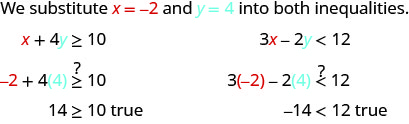
The ordered pair \((−2,4)\) made both inequalities true. Therefore \((−2,4)\) is a solution to this system.
b. Is the ordered pair \((3,1)\) a solution?
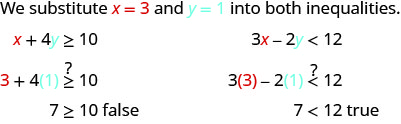
The ordered pair \((3,1)\) made one inequality true, but the other one false. Therefore \((3,1)\) is not a solution to this system.
Let's look at the graph for more insight. The red line and red shading represent \(x+4y\geq 10\). Any point that falls in the red region would be a solution to the given inequality. The blue line and blue shading represent \(3x-2y<12\). Any point that falls in the blue region would satisfy this inequality. The purple region satisfies both inequalities. Think about some other points. Would the point \((6.3)\) be a solution to the system of inequalities? Why or why not? What about the point of intersection between the two lines? Challenge yourself to choose a point that you know is a solution (or not) and practice using the equations to verify.

Solve a System of Linear Inequalities by Graphing
The solution to a single linear inequality is the region on one side of the boundary line that contains all the points that make the inequality true. The solution to a system of two linear inequalities is a region that contains the solutions to both inequalities. To find this region, we will graph each inequality separately and then locate the region where they are both true. The solution is always shown as a graph.
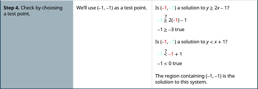
Solve the system by graphing: \(\left\{\begin{array} {l} y\geq 2x−1 \\ y<x+1\end{array}\right.\)
Solution:
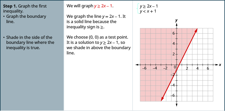
- Graph the first inequality.
- Graph the boundary line.
- Shade in the side of the boundary line where the inequality is true.
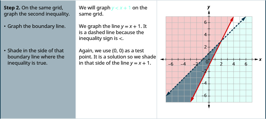
- On the same grid, graph the second inequality.
- Graph the boundary line.
- Shade in the side of that boundary line where the inequality is true.
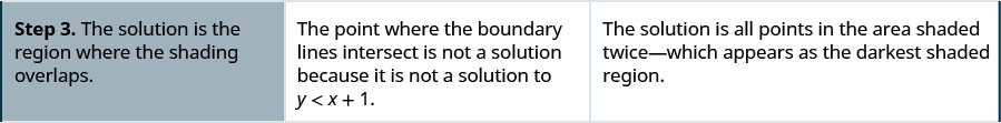
- The solution is the region where the shading overlaps.
- Check by choosing a test point.
a. Solve the system by graphing: \(\left\{\begin{array} {l} x−y>3\\y<−15x+4\end{array}\right.\)
- Answer
-
\(\left\{\begin{array} {l} x−y>3\\y<−15x+4\end{array}\right.\) Graph \(x - y > 3,\) by graphing \(x - y = 3\)
and testing a point.
The intercepts are \(x = 3\) and \(y = −3\) and the
boundary line will be dashed.
Test \((0, 0)\) which makes the inequality false so shade
(red) the side that does not contain \((0, 0).\)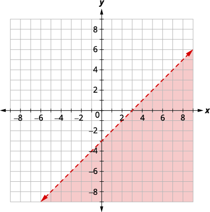
Graph \(y<−15x+4\) by graphing \(y=−15x+4\)
using the slope \(m=−15\) and \(y\)-intercept \(b = 4.\)
The boundary line will be dashed
Test \((0, 0)\) which makes the inequality true, so
shade (blue) the side that contains \((0, 0).\)
Choose a test point in the solution and verify that it is a solution to both inequalties.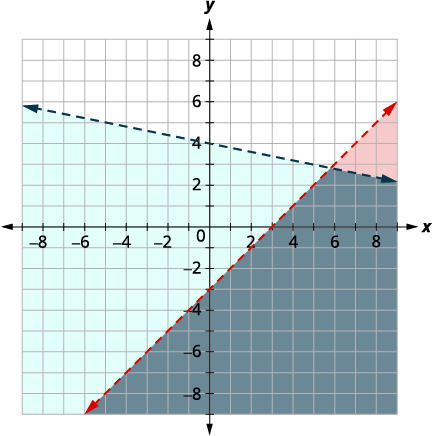
The point of intersection of the two lines is not included as both boundary lines were dashed. The solution is the area shaded twice—which appears as the darkest shaded region.
The solution is the grey region.
b. Solve the system by graphing: \(\left\{\begin{array} {l} x−2y<5\\y>−4\end{array}\right.\)
- Answer
-
\(\left\{\begin{array} {l} x−2y<5\\y>−4\end{array}\right.\) Graph \(x−2y<5\), by graphing \(x−2y=5\)
and testing a point. The intercepts are \(x = 5\) and \(y = −2.5\) and the
boundary line will be dashed.
Test \((0, 0)\) which makes the inequality true, so shade
(red) the side that contains \((0, 0).\)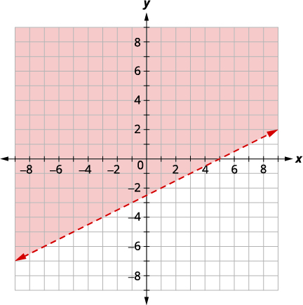
Graph \(y>−4\), by graphing \(y=−4\) and
recognizing that it is a horizontal line
through \(y=−4\). The boundary line will
be dashed.
Test \((0, 0)\) which makes the inequality
true so shade (blue) the side that contains \((0, 0).\)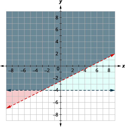
The point \((0,0)\) is in the solution and we have already found it to be a solution of each inequality. The point of intersection of the two lines is not included as both boundary lines were dashed.
The solution is the area shaded twice—which appears as the darkest shaded region.
The solution is the grey region.
c. Solve the system by graphing: \(\left\{\begin{array} {l} 4x+3y\geq 12 \\ y<−\frac{4}{3}x+1\end{array}\right.\)
- Answer
-
\(\left\{\begin{array} {l} 4x+3y\geq 12 \\ y<−\frac{4}{3}x+1\end{array}\right.\) Graph \(4x+3y\geq 12\), by graphing \(4x+3y=12\)
and testing a point. The intercepts are \(x = 3\)
and \(y = 4\) and the boundary line will be solid.
Test \((0, 0)\) which makes the inequality false, so
shade (red) the side that does not contain \((0, 0).\)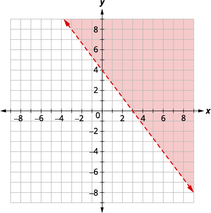
Graph \(y<−\frac{4}{3}x+1\) by graphing \(y=−\frac{4}{3}x+1\)
using the slope \(m=−\frac{4}{3}\) and \(y\)-intercept \(b = 1.\) The boundary line will be dashed.
Test \((0, 0)\) which makes the inequality true, so
shade (blue) the side that contains \((0, 0).\)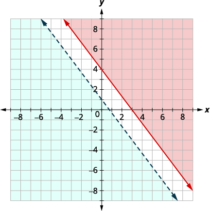
There is no point in both shaded regions, so the system has no solution.
Solve Applications of Systems of Inequalities
The first thing we’ll need to do to solve applications of systems of inequalities is to translate each condition into an inequality. Then we graph the system, as we did above, to see the region that contains the solutions. Many situations will be realistic only if both variables are positive, so we add inequalities to the system as additional requirements.
Christy sells her photographs at a booth at a street fair. At the start of the day, she wants to have at least 25 photos to display at her booth. Each small photo she displays costs her $4 and each large photo costs her $10. She doesn’t want to spend more than $200 on photos to display.
a. Write a system of inequalities to model this situation.
b. Graph the system.
c. Could she display 10 small and 20 large photos?
d. Could she display 20 large and 10 small photos?
Solution:
a.
\(\begin{array} {ll} \text{Let} &{x=\text{the number of small photos.}} \\ {} &{y=\text{the number of large photos}}\end{array}\)
To find the system of equations translate the information.
\( \qquad \begin{array} {l} \\ \\ \text{She wants to have at least 25 photos.} \\ \text{The number of small plus the number of large should be at least }25. \\ \hspace{45mm} x+y\geq 25 \\ \\ \\ $4 \text{ for each small and }$10\text{ for each large must be no more than }$200 \\ \hspace{40mm} 4x+10y\leq 200 \\ \\ \\ \text{The number of small photos must be greater than or equal to }0. \\ \hspace{50mm} x\geq 0 \\ \\ \\ \text{The number of large photos must be greater than or equal to }0. \\ \hspace{50mm} y\geq 0 \end{array} \)
We have our system of equations.
\(\hspace{65mm} \left\{\begin{array} {l} x+y\geq 25 \\4x+10y\leq 200\\x\geq 0\\y\geq 0\end{array}\right.\)
b.
Since \(x\geq 0\) and \(y\geq 0\) (both are greater than or equal to) all solutions will be in the first quadrant. As a result, our graph shows only quadrant one.
| To graph \(x+y\geq 25\), graph \(x+y=25\) as a solid line. Choose \((0, 0)\) as a test point. Since it does not make the inequality true, shade (red) the side that does not include the point \((0, 0).\) To graph \(4x+10y\leq 200\), graph \(4x+10y=200\) as a solid line. Choose \((0, 0)\) as a test point. Since it does make the inequality true, shade (blue) the side that include the point \((0, 0).\) |
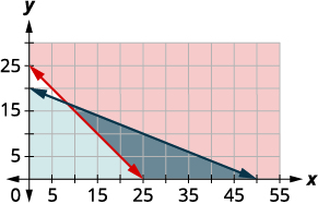 |
The solution of the system is the region of the graph that is shaded the darkest. The boundary line sections that border the darkly-shaded section are included in the solution as are the points on the \(x\)-axis from \((25, 0)\) to \((55, 0).\)
c. To determine if 10 small and 20 large photos would work, we look at the graph to see if the point \((10, 20)\) is in the solution region. We could also test the point to see if it is a solution of both equations.
It is not, Christy would not display 10 small and 20 large photos.
d. To determine if 20 small and 10 large photos would work, we look at the graph to see if the point \((20, 10)\) is in the solution region. We could also test the point to see if it is a solution of both equations.
It is, so Christy could choose to display 20 small and 10 large photos.
Notice that we could also test the possible solutions by substituting the values into each inequality.
When we use variables other than \(x\) and \(y\) to define an unknown quantity, we must change the names of the axes of the graph as well.
a. Omar needs to eat at least 800 calories before going to his team practice. All he wants is hamburgers and cookies, and he doesn’t want to spend more than $5. At the hamburger restaurant near his college, each hamburger has 240 calories and costs $1.40. Each cookie has 160 calories and costs $0.50.
a. Write a system of inequalities to model this situation.
b. Graph the system.
c. Could he eat 3 hamburgers and 1 cookie?
d. Could he eat 2 hamburgers and 4 cookies?
- Answer
-
a.
\(\begin{array} {ll} \text{Let} & h=\text{the number of hamburgers.} \\ & c=\text{the number of cookies}\end{array}\)To find the system of equations translate the information.
The calories from hamburgers at 240 calories each, plus the calories from cookies at 160 calories each must be more that 800.
\(\qquad \begin{array} {l} \hspace{40mm} 240h+160c\geq 800 \\ \\ \\ \text{The amount spent on hamburgers at }$1.40\text{ each, plus the amount spent on cookies}\\\text{at }$0.50\text{ each must be no more than }$5.00.\\ \hspace{40mm} 1.40h+0.50c\leq 5 \\ \\ \\ \text{The number of hamburgers must be greater than or equal to 0.} \\ \hspace{50mm} h\geq 0 \\ \text{The number of cookies must be greater than or equal to 0.}\\ \hspace{50mm} c\geq 0 \end{array} \)
\(\text{We have our system of equations.} \qquad \left\{ \begin{array} {l} 240h+160c\geq 800 \\ 1.40h+0.50c\leq 5 \\ h\geq 0 \\ c\geq 0\end{array} \right.\)
b.
Since \(h\geq 0\) and \(c\geq 0\) (both are greater than or equal to) all solutions will be in the first quadrant. As a result, our graph shows only quadrant one.To graph \(240h+160c\geq 800\), graph \(240h+160c=800\) as a solid line.
Choose \((0, 0)\) as a test point. Since it does not make the inequality true, shade (red) the side that does not include the point \((0, 0).\)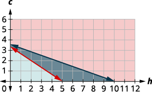
Graph \(1.40h+0.50c\leq 5\). The boundary line is \(1.40h+0.50c=5\). We test \((0, 0)\) and it makes the inequality true. We shade the side of the line that includes \((0, 0).\)
The solution of the system is the region of the graph that is shaded the darkest. The boundary line sections that border the darkly shaded section are included in the solution as are the points on the \(x\)-axis from \((5, 0)\) to \((10, 0).\)
c. To determine if 3 hamburgers and 2 cookies would meet Omar’s criteria, we see if the point \((3, 2)\) is in the solution region. It is, so Omar might choose to eat 3 hamburgers and 2 cookies.
d. To determine if 2 hamburgers and 4 cookies would meet Omar’s criteria, we see if the point \((2, 4)\) is in the solution region. It is, Omar might choose to eat 2 hamburgers and 4 cookies.
We could also test the possible solutions by substituting the values into each inequality.
Key Concepts
- Solutions of a System of Linear Inequalities: Solutions of a system of linear inequalities are the values of the variables that make all the inequalities true. The solution of a system of linear inequalities is shown as a shaded region in the \(xy\)-coordinate system that includes all the points whose ordered pairs make the inequalities true.
- How to solve a system of linear inequalities by graphing.
- Graph the first inequality.
Graph the boundary line.
Shade in the side of the boundary line where the inequality is true. - On the same grid, graph the second inequality.
Graph the boundary line.
Shade in the side of that boundary line where the inequality is true. - The solution is the region where the shading overlaps.
- Check by choosing a test point.
- Graph the first inequality.