4.1: Exponential Functions

Learning Objectives

• Evaluate exponential functions.
• Find the equation of an exponential function.
• Use compound interest formulas.
• Evaluate exponential functions with base \(e\).

The game of chess is believed to have begun in 6th century India as a battle field simulation game.  However, another famous legend claims that the grand vizier to King Shihram, Sissa ben Dahir, invented the game to bring attention to the kings faults without totally offending him.  The game was created so that the King was the most important piece but it could do nothing without the help of the other pieces.  King Shihram was so impressed by the game and its teachings that he granted a wish to the vizier to show his gratitude. Sissa ben Dahir only asked for “One grain of rice, representing the first square of a chessboard. Two grains for the second square. Four grains for the next. Then eight, 16, 32… doubling for each successive square until the 64th and last square is counted.”  Legend has it that the Kind was pleased with the humble request and granted it immediately.  Was this a good idea?

We might say that Sissa ben Dahir's grains of wheat is “exponential” growth, meaning that something is growing very rapidly. To a mathematician, however, the term exponential growth has a very specific meaning. In this section, we will take a look at exponential functions, which model this kind of rapid growth..

Defining an Exponential Function

When exploring linear growth, we observed a constant rate of change—a constant number by which the output (y-value) increased for each unit increase in input (x-value). For example, in the equation \(f(x)=3x+4\), the slope indicates that the output increases by \(3\) for every \(1\) unit increase in the input. The scenario with the grains of wheat example is different because we have a percent change per unit time (rather than a constant change) in the number of people.

A study found that the percentage of the population who owned a cellphone in \(1990\) was just \(2%\). In \(2025\), there are more cellphones than people with nearly \(98%\) of the population owning a smartphone. Throughout this time period, cell phone ownership grew exponentially.  The current growth rate is around \(6%\) as we are nearing saturation. 

What exactly does it mean to grow exponentially? What does the word double have in common with percent increase? People toss these words around errantly. Are these words used correctly? The words certainly appear frequently in the media.

• Percent change refers to a change based on a percent of the original amount.
• Exponential growth refers to an increase based on a constant multiplicative rate of change over equal increments of time, that is, a percent increase of the original amount over time.
• Exponential decay refers to a decrease based on a constant multiplicative rate of change over equal increments of time, that is, a percent decrease of the original amount over time.

For us to gain a clear understanding of exponential growth, let's contrast exponential growth with linear growth. Say we have two functions. The first function is exponential, starting with an input of \(0\),increasingrease each input by \(1\) (as shown in Table \(\PageIndex{1}\) below). Notice the pattern of outputs?  Each output is double the previous one.  The second function is linear, starting with an input of \(0\),follows the same pattern of increasing each input by \(1\). Notice the pattern of outputs?  Instead of doubling the previous output, we are increasing the previous output by adding \(2\) to the corresponding consecutive outputs.  One could also say that the input is doubling.  Looking at the Table, one can easily see how exponential growth increases much faster than linear growth.  

From Table \(\PageIndex{1}\) we can infer that for these two functions, exponential growth far surpasses linear growth.

• Exponential growth refers to the original value from the range increases by the same percentage over equal increments found in the domain.
• Linear growth refers to the original value from the range increases by the same amount over equal increments found in the domain.

Table \(\PageIndex{1}\)

\(x\)	\(f(x)=2^x\)	\(g(x)=2x\)
\(0\)	\(1\)	\(0\)
\(1\)	\(2\)	\(2\)
\(2\)	\(4\)	\(4\)
\(3\)	\(8\)	\(6\)
\(4\)	\(16\)	\(8\)
\(5\)	\(32\)	\(10\)
\(6\)	\(64\)	\(12\)

Apparently, the difference between “the same percentage” and “the same amount” is quite significant. For exponential growth, over equal increments, the constant multiplicative rate of change resulted in doubling the output whenever the input increased by one. For linear growth, the constant additive rate of change over equal increments resulted in adding \(2\) to the output whenever the input was increased by one.

The general form of the exponential function is \(f(x)=ab^x\), where \(a\) is any nonzero number, \(b\) is a positive real number not equal to \(1\).

• If \(b>1\),the function grows at a rate proportional to its size.
• If \(0<b<1\), the function decays at a rate proportional to its size.

Let’s look at the function \(f(x)=2^x\) from our example. We will create a table (Table \(\PageIndex{2}\)) to determine the corresponding outputs over an interval in the domain from \(−3\) to \(3\).

Table \(\PageIndex{2}\)

\(x\)	\(−3\)	\(−2\)	\(−1\)	\(0\)	\(1\)	\(2\)	\(3\)
\(f(x)=2^x\)	\(2^{−3}=\dfrac{1}{8}\)	\(2^{−2}=\dfrac{1}{4}\)	\(2^{−1}=\dfrac{1}{2}\)	\(2^0=1\)	\(2^1=2\)	\(2^2=4\)	\(2^3=8\)

Let us examine the graph of \(f\) by plotting the ordered pairs from Table \(\PageIndex{2}\) and then make a few observations \(\PageIndex{1}\).

Figure \(\PageIndex{1}\)

Let’s define the behavior of the graph of the exponential function \(f(x)=2^x\) and highlight some its key characteristics.

• the domain is \((−\infty,\infty)\),
• the range is \((0,\infty)\),
• as \(x\rightarrow \infty\), \(f(x)\rightarrow \infty\),
• as \(x\rightarrow −\infty\), \(f(x)\rightarrow 0\),
• \(f(x)\) is always increasing,
• the graph of \(f(x)\) will never touch the x-axis because base two raised to any exponent never has the result of zero.
• \(y=0\) is the horizontal asymptote.
• the y-intercept is \(1\).

Example \(\PageIndex{1}\): Identifying Exponential Functions

Which of the following equations are not exponential functions?

• \(f(x)=4^{3(x−2)}\)
• \(g(x)=x^3\)
• \(h(x)=\left(\dfrac{1}{3}\right)^x\)
• \(j(x)=(−2)^x\)

Solution

By definition, an exponential function has a constant as a base and an independent variable as an exponent. Thus, \(g(x)=x^3\) does not represent an exponential function because the base is an independent variable. In fact, \(g(x)=x^3\) is a power function.

Recall that the base \(b\) of an exponential function is always a positive constant, and \(b≠1\). Thus, \(j(x)={(−2)}^x\) does not represent an exponential function because the base, \(−2\), is less than \(0\).

Evaluating Exponential Functions

Recall that the base of an exponential function must be a positive real number other than \(1\).Why do we limit the base b to positive values? To ensure that the outputs will be real numbers. Observe what happens if the base is not positive:

• Let \(b=−9\) and \(x=\dfrac{1}{2}\). Then \(f(x)=f\left(\dfrac{1}{2}\right)={(−9)}^{\dfrac{1}{2}}=\sqrt{−9}\),which is not a real number.

Why do we limit the base to positive values other than \(1\)? Because base \(1\) results in the constant function. Observe what happens if the base is \(1\):

• Let \(b=1\). Then \(f(x)=1^x=1\) for any value of \(x\).

To evaluate an exponential function with the form \(f(x)=b^x\),we simply substitute \(x\) with the given value, and calculate the resulting power. For example:

Let \(f(x)=2^x\). What is \(f(3)\)?

\[\begin{align*} f(x)&= 2^x\\ f(3)&= 2^3 \qquad \text{Substitute } x=3\\ &= 8 \qquad \text{Evaluate the power} \end{align*}\]

To evaluate an exponential function with a form other than the basic form, it is important to follow the order of operations. For example:

Let \(f(x)=30{(2)}^x\). What is \(f(3)\)?

\[\begin{align*} f(x)&= 30{(2)}^x\\ f(3)&= 30{(2)}^3 \qquad \text{Substitute } x=3\\ &= 30(8) \qquad \text{Simplify the power first}\\ &= 240 \qquad \text{Multiply} \end{align*}\]

Note that if the order of operations were not followed, the result would be incorrect:

\[f(3)=30{(2)}^3≠{60}^3=216,000 \nonumber\]

Example \(\PageIndex{2}\): Evaluating Exponential Functions

Let \(f(x)=5{(3)}^{x+1}\). Evaluate \(f(2)\) without using a calculator.

Solution

Follow the order of operations. Be sure to pay attention to the parentheses.

\[\begin{align*} f(x)&= 5{(3)}^{x+1}\\ f(2)&= 5{(3)}^{2+1} \qquad \text{Substitute } x=2\\ &= 5{(3)}^3 \qquad \text{Add the exponents}\\ &= 5(27) \qquad \text{Simplify the power}\\ &= 135 \qquad \text{Multiply} \end{align*}\]

Defining Exponential Growth/Decay

Because the output of exponential functions increases very rapidly, the term “exponential growth” is often used in everyday language to describe anything that grows or increases rapidly. However, exponential growth can be defined more precisely in a mathematical sense. If the growth rate is proportional to the amount present, the function models exponential growth.

A function that models exponential growth grows by a rate proportional to the amount present. For any real number \(x\) and any positive real numbers \(a\) and \(b\) such that \(b≠1\),an exponential growth function has the form

\[f(x)=ab^x\]

where

• \(a\) is the initial or starting value of the function.
• \(b\) is the growth factor or growth multiplier per unit \(x\).
  • If \(b>1\) the function models exponential growth.
  • If \(0<b<1\), the function models exponential decay.  

In more general terms, we have an exponential function, in which a constant base is raised to a variable exponent. To differentiate between linear and exponential functions, let’s consider two companies, A and B. Company A has \(100\) stores and expands by opening \(50\) new stores a year, so its growth can be represented by the function \(A(x)=100+50x\). Company B has \(100\) stores and expands by increasing the number of stores by \(50\%\) each year, so its growth can be represented by the function \(B(x)=100{(1+0.5)}^x\). We take half of the previous amount each year and add it to that amount.  Notice how the increase between of the y-value each year for Company B is not constant. 

Table \(\PageIndex{3}\) illustrates a few years of growth for these companies.

Table \(\PageIndex{3}\)

Year, \(x\)	Stores, Company A	Stores, Company B
\(0\)	\(100+50(0)=100\)	\(100{(1+0.5)}^0=100\)
\(1\)	\(100+50(1)=150\)	\(100{(1+0.5)}^1=150\)
\(2\)	\(100+50(2)=200\)	\(100{(1+0.5)}^2=225\)
\(3\)	\(100+50(3)=250\)	\(100{(1+0.5)}^3=337.5\)
\(x\)	\(A(x)=100+50x\)	\(B(x)=100{(1+0.5)}^x\)

The graphs comparing the number of stores for each company over a five-year period are shown in Figure \(\PageIndex{2}\). We can see that, with exponential growth, the number of stores increases much more rapidly than with linear growth.

Figure \(\PageIndex{2}\): The graph shows the numbers of stores Companies A and B opened over a five-year period.

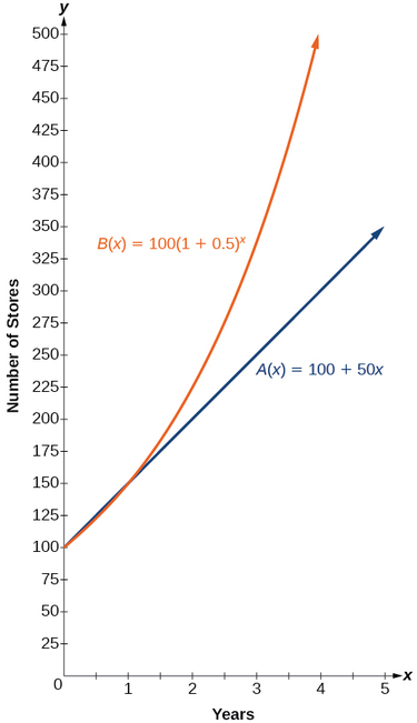
Notice that the domain for both functions is \([0,\infty)\),and the range for both functions is \([100,\infty)\). After year 1, Company B always has more stores than Company A.

Now we will turn our attention to the function representing the number of stores for Company \(B\), \(B(x)=100{(1+0.5)}^x\). In this exponential function, \(100\) represents the initial number of stores, \(0.50\) represents the growth rate, and \(1+0.5=1.5\) represents the growth factor. Generalizing further, we can write this function as \(B(x)=100{(1.5)}^x\),where \(100\) is the initial value, \(1.5\) is called the base, and \(x\) is called the exponent.

Example \(\PageIndex{3}\): Evaluating a Real-World Exponential Model

At the beginning of this section, we learned that the population of India was about \(1.25\) billion in the year 2013, with an annual growth rate of about \(1.2\%\). This situation is represented by the growth function \(P(t)=1.25{(1.012)}^t\), where \(t\) is the number of years since 2013. To the nearest thousandth, what will the population of India be in 2031?

Solution

To estimate the population in 2031, we evaluate the models for \(t=18\), because 2031 is \(18\) years after 2013. Rounding to the nearest thousandth,

\[P(18)=1.25{(1.012)}^{18}≈1.549 \nonumber\]

There will be about \(1.549\) billion people in India in the year 2031.

Example \(\PageIndex{4}\)

If a medicine has a four-hour half-life, about \(100\) mg will remain in your system after four hours from a \(200\) mg dose.  Around \(50\) mg will be left after another \(4\) hours or (\(8\) hours total). This helps doctors determine the appropriate dosage of medications in a safe and effective manner.  How much of the medicine will be left in the body after \(16\) hours?

Solution

Time after medication was administered	Amount of medication in the bloodstream.
\(0\)	\(200\) mg
\(4\)	\(100\) mg
\(8\)	\(50\) mg
\(12\)	\(25\) mg
\(16\)	\(12.5\) mg

We can see that the amount of medication decreases by one-half of the previous amount after each \(4\) hour time period. This solution is very easy to determine with a table of values.  However, suppose we were to write the exponential function. In that case, we notice that the initial amount of medication is \(200\) mg and the rate of decrease is \(\frac{1}{2}\), resulting in the equation \[f(x)=200(\frac{1}{2})b^x\] where x is the number of time periods. 

One can see that the shape of the exponential decay graph is similar to that of exponential growth. 

Finding Equations of Exponential Functions

In the previous examples, we were given an exponential function, which we then evaluated for a given input. Sometimes we are given information about an exponential function without knowing the function explicitly. We must use the information to first write the form of the function, then determine the constants \(a\) and \(b\),and evaluate the function.

Example \(\PageIndex{5}\): Writing an Exponential Model When the Initial Value Is Known

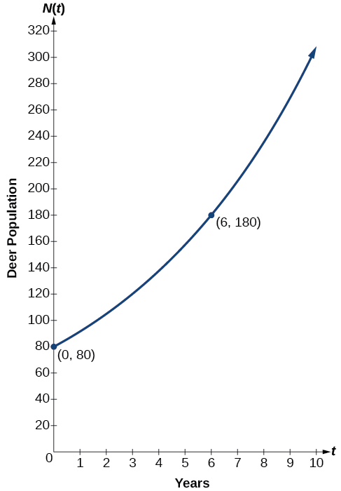
In 2006, \(80\) deer were introduced into a wildlife refuge. By 2012, the population had grown to \(180\) deer. The population was growing exponentially. Write an algebraic function \(N(t)\) representing the population \((N)\) of deer over time \(t\).

Solution

We let our independent variable \(t\) be the number of years after 2006. Thus, the information given in the problem can be written as input-output pairs: (0, 80) and (6, 180). Notice that by choosing our input variable to be measured as years after 2006, we have given ourselves the initial value for the function, \(a=80\). We can now substitute the second point into the equation \(N(t)=80b^t\) to find \(b\):

\[\begin{align*} N(t)&= 80b^t\\ 180&= 80b^6 \qquad \text{Substitute using point } (6, 180)\\ \dfrac{9}{4}&= b^6 \qquad \text{Divide and write in lowest terms}\\ b&= {\left (\dfrac{9}{4} \right )}^{\tfrac{1}{6}} \qquad \text{Isolate b using properties of exponents}\\ b&\approx 1.1447 \qquad \text{Round to 4 decimal places} \end{align*}\]

Unless otherwise stated, do not round any intermediate calculations. Then round the final answer to four places for the remainder of this section.

The exponential model for the population of deer is \(N(t)=80{(1.1447)}^t\). (Note that this exponential function models short-term growth. As the inputs gets large, the output will get increasingly larger, so much so that the model may not be useful in the long term.)

We can graph our model to observe the population growth of deer in the refuge over time. Notice that the graph in Figure \(\PageIndex{3}\) passes through the initial points given in the problem, \((0, 80)\) and \((6, 180)\). We can also see that the domain for the function is \([0,\infty)\),and the range for the function is \([80,\infty)\).

Figure \(\PageIndex{3}\): Graph showing the population of deer over time, \(N(t)=80{(1.1447)}^t\), \(t\) years after 2006

Example \(\PageIndex{6}\): Writing an Exponential Model When the Initial Value is Not Known

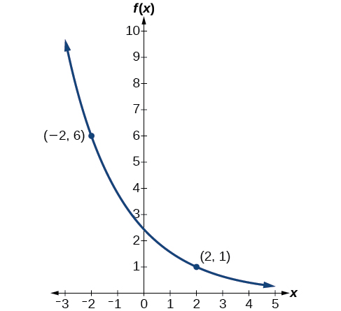
Find an exponential function that passes through the points \((−2,6)\) and \((2,1)\).

Solution

Because we don’t have the initial value, we substitute both points into an equation of the form \(f(x)=ab^x\), and then solve the system for \(a\) and \(b\).

• Substituting \((−2,6)\) gives \(6=ab^{−2}\)
• Substituting \((2,1)\) gives \(1=ab^2\)

Use the first equation to solve for \(a\) in terms of \(b\):

\[\begin{align*} 6&= ab^{-2}\\ \dfrac{6}{b^{-2}}&= a \qquad \text{Divide}\\ a&= 6b^2 \qquad \text{Use properties of exponents to rewrite the denominator} \end{align*}\]

Substitute a in the second equation, and solve for \(b\):

\[\begin{align*} 1&= ab^{2}\\ 1&= 6b^2 b^2\\ &= 6b^4 \qquad \text{Substitute a}\\ b&= \left (\dfrac{1}{6} \right )^{\tfrac{1}{4}} \qquad \text{Round 4 decimal places rewrite the denominator}\\ b&\approx 0.6389 \end{align*}\]

Use the value of \(b\) in the first equation to solve for the value of \(a\):

\[\begin{align*} a&= 6b^{2}\\ &\approx 6(0.6389)^2 \\ &\approx 2.4492 \end{align*}\]

Thus, the equation is \(f(x)=2.4492{(0.6389)}^x\).

We can graph our model to check our work. Notice that the graph in Figure \(\PageIndex{4}\) passes through the initial points given in the problem, \((−2, 6)\) and \((2, 1)\). The graph is an example of an exponential decay function.

Figure \(\PageIndex{4}\): The graph of \(f(x)=2.4492{(0.6389)}^x\) models exponential decay.

Q&A: Do two points always determine a unique exponential function?

Yes, provided the two points are either both above the x-axis or both below the x-axis and have different x-coordinates. But keep in mind that we also need to know that the graph is, in fact, an exponential function. Not every graph that looks exponential really is exponential. We need to know the graph is based on a model that shows the same percent growth with each unit increase in \(x\), which in many real world cases involves time.

Example \(\PageIndex{7}\): Writing an Exponential Function Given Its Graph

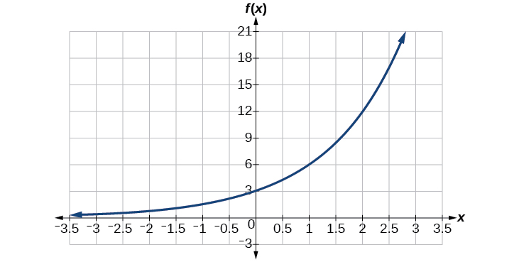
Find an equation for the exponential function graphed in Figure \(\PageIndex{5}\).

Figure \(\PageIndex{5}\)

Solution

We can choose the \(y\)-intercept of the graph, \((0,3)\), as our first point. This gives us the initial value, \(a=3\). Next, choose a point on the curve some distance away from \((0,3)\) that has integer coordinates. One such point is \((2,12)\).

\[\begin{align*} y&= ab^x \qquad \text{Write the general form of an exponential equation}\\ y&= 3b^x \qquad \text{Substitute the initial value } 3 \text{ for } a\\ 12&= 3b^2 \qquad \text{Substitute in 12 for } y \text{ and } 2 \text{ for } x\\ 4&= b^2 \qquad \text{Divide by }3\\ b&= \pm 2 \qquad \text{Take the square root} \end{align*}\]

Because we restrict ourselves to positive values of \(b\), we will use \(b=2\). Substitute \(a\) and \(b\) into the standard form to yield the equation \(f(x)=3{(2)}^x\).

Key Equations

definition of the exponential function	\(f(x)=b^x\), where \(b>0\), \(b≠1\)
definition of exponential growth	\(f(x)=ab^x\), where \(a>0\), \(b>0\), \(b≠1\)

Key Concepts

• An exponential function is defined as a function with a positive constant other than \(1\) raised to a variable exponent. 
• A function is evaluated by solving at a specific value. 
• An exponential model can be found when the growth rate and initial value are known. 
• An exponential model can be found when the two data points from the model are known. 
• An exponential model can be found using two data points from the graph of the model. 
• An exponential model can be found using two data points from the graph and a calculator. 
• The number \(e\) is a mathematical constant often used as the base of real world exponential growth and decay models. Its decimal approximation is \(e≈2.718282\).
• Scientific and graphing calculators have the key \([ex]\) or \([exp(x)]\) for calculating powers of \(e\). 
• Continuous growth or decay models are exponential models that use \(e\) as the base. Continuous growth and decay models can be found when the initial value and growth or decay rate are known.