3.1: Basic Differentiation Rules

Learning Objectives

• State the constant, constant multiple, and power rules.
• Apply the sum and difference rules to combine derivatives.

Finding derivatives of functions by using the definition of the derivative can be a lengthy and, for certain functions, a rather challenging process. For example, previously we found that

\[\dfrac{d}{dx}\left(\sqrt{x}\right)=\dfrac{1}{2\sqrt{x}} \nonumber \]

by using a process that involved multiplying an expression by a conjugate prior to evaluating a limit.

The process that we could use to evaluate \(\dfrac{d}{dx}\left(\sqrt[3]{x}\right)\) using the definition, while similar, is more complicated.

In this section, we develop rules for finding derivatives that allow us to bypass this process. We begin with the basics.

The Basic Rules

The functions \(f(x)=c\) and \(g(x)=x^n\) where \(n\) is a positive integer are the building blocks from which all polynomials and rational functions are constructed. To find derivatives of polynomials and rational functions efficiently without resorting to the limit definition of the derivative, we must first develop formulas for differentiating these basic functions.

The Constant Rule

We first apply the limit definition of the derivative to find the derivative of the constant function, \(f(x)=c\). For this function, both \(f(x)=c\) and \(f(x+h)=c\), so we obtain the following result:

\[\begin{align*} f′(x) &=\lim_{h→0} \dfrac{f(x+h)−f(x)}{h} \\[4pt] &=\lim_{h→0}\dfrac{c−c}{h} \\[4pt] &=\lim_{h→0}\dfrac{0}{h} \\[4pt] &=\lim_{h→0}0=0 \end{align*}\]

The rule for differentiating constant functions is called the constant rule. It states that the derivative of a constant function is zero; that is, since a constant function is a horizontal line, the slope, or the rate of change, of a constant function is \(0\). We restate this rule in the following theorem.

The Constant Rule

Let \(c\) be a constant. If \(f(x)=c\), then \(f′(x)=0.\)

Alternatively, we may express this rule as

\[\dfrac{d}{dx}(c)=0 \nonumber \]

Example \(\PageIndex{1}\): Applying the Constant Rule

Find the derivative of \(f(x)=8\)

Solution

This is just a one-step application of the rule: \(\boxed{f′(x)=0}\).

Exercise \(\PageIndex{1}\)

Find the derivative of \(g(x)=−3\)

Answer

0

The Power Rule

We have shown that

\[\dfrac{d}{dx}\left(x^2\right)=2x\quad\text{ and }\quad\dfrac{d}{dx}\left(x^{\frac{1}{2}}\right)=\dfrac{1}{2}x^{−\frac{1}{2}} \nonumber \]

At this point, you might see a pattern beginning to develop for derivatives of the form \(\dfrac{d}{dx}\left(x^n\right)\). We continue our examination of derivative formulas by differentiating power functions of the form \(f(x)=x^n\) where \(n\) is a positive integer. We develop formulas for derivatives of this type of function in stages, beginning with positive integer powers. Before stating and proving the general rule for derivatives of functions of this form, we take a look at a specific case, \(\dfrac{d}{dx}(x^3)\). As we go through this derivation, pay special attention to the portion of the expression in boldface, as the technique used in this case is essentially the same as the technique used to prove the general case.

Example \(\PageIndex{2}\): Differentiating \(x^3\)

Find \(\dfrac{d}{dx}\left(x^3\right)\)

Solution:

\[ \begin{align*}  \dfrac{d}{dx}\left(x^3\right)& =\lim_{h→0}\dfrac{(x+h)^3−x^3}{h}   \\[4pt] & = \lim_{h→0}\dfrac{x^3+3x^2h+3xh^2+h^3−x^3}{h}  \\[4pt] & = \lim_{h→0}\dfrac{3x^2h+3xh^2+h^3}{h} \\[4pt] & =\lim_{h→0}\dfrac{h(3x^2+3xh+h^2)}{h} \\[4pt] & = \lim_{h→0}(3x^2+3xh+h^2)  \\[4pt] & = \boxed{3x^2} \end{align*} \]

Exercise \(\PageIndex{2}\)

Find \(\dfrac{d}{dx}\left(x^4\right)\)

Hint

Use \((x+h)^4=x^4+4x^3h+6x^2h^2+4xh^3+h^4\) and follow the procedure outlined in the preceding example.

Answer

\(\dfrac{d}{dx}\left(x^4\right) = 4x^3\)

As we shall see, the procedure for finding the derivative of the general form \(f(x)=x^n\) is very similar. Although it is often unwise to draw general conclusions from specific examples, we note that when we differentiate \(f(x)=x^3\), the power on \(x\) becomes the coefficient of \(x^2\) in the derivative and the power on \(x\) in the derivative decreases by 1. The following theorem states that the power rule holds for all positive integer powers of \(x\). We will eventually extend this result to negative integer powers. Later, we will see that this rule may also be extended first to rational powers of \(x\) and then to arbitrary powers of \(x\). Be aware, however, that this rule does not apply to functions in which a constant is raised to a variable power, such as \(f(x)=3^x\).

The Power Rule

Let \(n\) be a positive integer. If \(f(x)=x^n\),then

\[f′(x)=nx^{n−1} \nonumber \]

Alternatively, we may express this rule as

\[\dfrac{d}{dx}\left(x^n\right)=nx^{n−1} \nonumber \]

Proof

For \(f(x)=x^n\) where \(n\) is a positive integer, we have

\[f′(x)=\lim_{h→0}\dfrac{(x+h)^n−x^n}{h} \nonumber \]

Since

\((x+h)^n=x^n+nx^{n−1}h+\binom{n}{2}x^{n−2}h^2+\binom{n}{3}x^{n−3}h^3+…+nxh^{n−1}+h^n\)

we see that

\((x+h)^n−x^n=nx^{n−1}h+\binom{n}{2}x^{n−2}h^2+\binom{n}{3}x^{n−3}h^3+…+nxh^{n−1}+h^n\)

Next, divide both sides by h:

\(\dfrac{(x+h)^n−x^n}{h}=\dfrac{nx^{n−1}h+\binom{n}{2}x^{n−2}h^2+\binom{n}{3}x^{n−3}h^3+…+nxh^{n−1}+h^n}{h}\)

Thus,

\(\dfrac{(x+h)^n−x^n}{h}=nx^{n−1}+\binom{n}{2}x^{n−2}h+\binom{n}{3}x^{n−3}h^2+…+nxh^{n−2}+h^{n−1}\)

Finally,

\[f′(x)=\lim_{h→0}\left(nx^{n−1}+\binom{n}{2}x^{n−2}h+\binom{n}{3}x^{n−3}h^2+…+nxh^{n−2}+h^{n-1}\right) \nonumber \]

\(=nx^{n−1}\)

□

Example \(\PageIndex{3}\): Applying the Power Rule

Find the derivative of the function \(f(x)=x^{10}\) by applying the power rule.

Solution

Using the power rule with \(n=10\), we obtain

\[f'(x)=10x^{10−1}=\boxed{10x^9} \nonumber \]

Exercise \(\PageIndex{3}\)

Find the derivative of \(f(x)=x^7\)

Hint

Use the power rule with \(n=7\).

Answer

\(f′(x)=7x^6\)

The Sum, Difference, and Constant Multiple Rules

We find our next differentiation rules by looking at derivatives of sums, differences, and constant multiples of functions. Just as when we work with functions, there are rules that make it easier to find derivatives of functions that we add, subtract, or multiply by a constant. These rules are summarized in the following theorem.

Sum, Difference, and Constant Multiple Rules

Let \(f(x)\) and \(g(x)\) be differentiable functions and \(k\) be a constant. Then each of the following equations holds.

Sum Rule. The derivative of the sum of a function \(f\) and a function \(g\) is the same as the sum of the derivative of \(f\) and the derivative of \(g\).

\[\dfrac{d}{dx}\big(f(x)+g(x)\big)=\dfrac{d}{dx}\big(f(x)\big)+\dfrac{d}{dx}\left(g(x)\right) \nonumber \]

that is,

\[\text{for }s(x)=f(x)+g(x),\quad s′(x)=f′(x)+g′(x) \nonumber \]

Difference Rule. The derivative of the difference of a function \(f\) and a function \(g\) is the same as the difference of the derivative of \(f\) and the derivative of \(g\) :

\[\dfrac{d}{dx}\left(f(x)−g(x)\right)=\dfrac{d}{dx}(f(x))−\dfrac{d}{dx}(g(x)) \nonumber \]

that is,

\[\text{for }d(x)=f(x)−g(x),\quad d′(x)=f′(x)−g′(x) \nonumber \]

Constant Multiple Rule. The derivative of a constant \(k\) multiplied by a function \(f\) is the same as the constant multiplied by the derivative:

\[\dfrac{d}{dx}\left(kf(x)\right)=k\dfrac{d}{dx}\left(f(x)\right) \nonumber \]

that is,

\[\text{for }m(x)=kf(x),\quad m′(x)=kf′(x) \nonumber \]

Proof

We provide only the proof of the sum rule here. The rest follow in a similar manner.

For differentiable functions \(f(x)\) and \(g(x)\), we set \(s(x)=f(x)+g(x)\). Using the limit definition of the derivative we have

\[s′(x)=\lim_{h→0}\dfrac{s(x+h)−s(x)}{h}\nonumber \]

By substituting \(s(x+h)=f(x+h)+g(x+h)\) and \(s(x)=f(x)+g(x),\) we obtain

\[s′(x)=\lim_{h→0}\dfrac{\big(f(x+h)+g(x+h)\big)−\big(f(x)+g(x)\big)}{h}\nonumber \]

Rearranging and regrouping the terms, we have

\[s′(x)=\lim_{h→0}\left(\dfrac{f(x+h)−f(x)}{h}+\dfrac{g(x+h)−g(x)}{h}\right)\nonumber \]

We now apply the sum law for limits and the definition of the derivative to obtain

\[s′(x)=\lim_{h→0}\dfrac{f(x+h)−f(x)}{h}+\lim_{h→0}\dfrac{g(x+h)−g(x)}{h}=f′(x)+g′(x)\nonumber \]

□

Example \(\PageIndex{4}\): Applying the Constant Multiple Rule

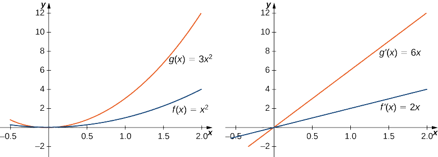
Find the derivative of \(g(x)=3x^2\) and compare it to the derivative of \(f(x)=x^2\).

Solution

We use the power rule directly:

\[g′(x)=\dfrac{d}{dx}(3x^2)=3\dfrac{d}{dx}(x^2)=3(2x)=6x\nonumber \]

Since \(f(x)=x^2\) has derivative \(f′(x)=2x\), we see that the derivative of \(g(x)\) is 3 times the derivative of \(f(x)\). This relationship is illustrated in Figure \(\PageIndex{1}\).

Figure \(\PageIndex{1}\): The derivative of \(g(x)\) is 3 times the derivative of \(f(x)\).

Example \(\PageIndex{5}\): Applying Basic Derivative Rules

Find the derivative of \(f(x)=2x^5+7\)

Solution

We begin by applying the rule for differentiating the sum of two functions, followed by the rules for differentiating constant multiples of functions and the rule for differentiating powers. To better understand the sequence in which the differentiation rules are applied, we use Leibniz notation throughout the solution:

\[\begin{align*} f′(x)&=\dfrac{d}{dx}\left(2x^5+7\right)\\[4pt]
&=\dfrac{d}{dx}(2x^5)+\dfrac{d}{dx}(7) & & \text{Apply the sum rule.}\\[4pt]
&=2\dfrac{d}{dx}(x^5)+\dfrac{d}{dx}(7) & & \text{Apply the constant multiple rule.}\\[4pt]
&=2(5x^4)+0 & & \text{Apply the power rule and the constant rule.}\\[4pt]
&=\boxed{10x^4} & & \text{Simplify.} \end{align*}\]

Exercise \(\PageIndex{4}\)

Find the derivative of \(f(x)=2x^3−6x^2+3\)

Hint

Use the preceding example as a guide.

Answer

\(f′(x)=6x^2−12x\)

Example \(\PageIndex{6}\): Finding the Equation of a Tangent Line

Find the equation of the line tangent to the graph of \(f(x)=x^2−4x+6\) at \(x=1\)

Solution

To find the equation of the tangent line, we need a point and a slope. To find the point, compute

\[f(1)=1^2−4(1)+6=3 \nonumber \]

This gives us the point \((1,3)\). Since the slope of the tangent line at 1 is \(f′(1)\), we must first find \(f′(x)\). Using the definition of a derivative, we have

\[f′(x)=2x−4\nonumber \]

so the slope of the tangent line is \(f′(1)=−2\). Using the point-slope formula, we see that the equation of the tangent line is

\[y−3=-2(x−1)\nonumber \]

Putting the equation of the line in slope-intercept form, we obtain

\[\boxed{y=-2x+5}\nonumber \]

Exercise \(\PageIndex{5}\)

Find the equation of the line tangent to the graph of \(f(x)=3x^2−11\) at \(x=2\). Use the point-slope form.

Hint

Use the preceding example as a guide.

Answer

\(y=12x−23\)

Derivative of the Exponential Function

Just as when we found the derivatives of other functions, we can find the derivatives of exponential and logarithmic functions using formulas. As we develop these formulas, we need to make certain basic assumptions. The proofs that these assumptions hold are beyond the scope of this course.

First of all, we begin with the assumption that the function \(B(x)=b^x,\, b>0,\) is defined for every real number and is continuous. In previous courses, the values of exponential functions for all rational numbers were defined—beginning with the definition of \(b^n\), where \(n\) is a positive integer—as the product of \(b\) multiplied by itself \(n\) times. Later, we defined \(b^0=1,b^{−n}=\dfrac{1}{b^n}\), for a positive integer \(n\), and \(b^{\frac{s}{t}}=(\sqrt[t]{b})^s\) for positive integers \(s\) and \(t\). These definitions leave open the question of the value of \(b^r\) where \(r\) is an arbitrary real number. By assuming the continuity of \(B(x)=b^x,b>0\), we may interpret \(b^r\) as \(\displaystyle \lim_{x→r}b^x\) where the values of \(x\) as we take the limit are rational. For example, we may view \(4^π\) as the number satisfying

\[4^3<4^π<4^4,\quad 4^{3.1}<4^π<4^{3.2},\quad 4^{3.14}<4^π<4^{3.15}, \quad 4^{3.141}<4^{π}<4^{3.142},\quad 4^{3.1415}<4^{π}<4^{3.1416},\quad … \nonumber \]

As we see in the following table, \(4^π≈77.88.\)

\(x\)	\(4^x\)	\(x\)	\(4^x\)
\(4^3\)	64	\(4^{3.141593}\)	77.8802710486
\(4^{3.1}\)	73.5166947198	\(4^{3.1416}\)	77.8810268071
\(4^{3.14}\)	77.7084726013	\(4^{3.142}\)	77.9242251944
\(4^{3.141}\)	77.8162741237	\(4^{3.15}\)	78.7932424541
\(4^{3.1415}\)	77.8702309526	\(4^{3.2}\)	84.4485062895
\(4^{3.14159}\)	77.8799471543	\(4^{4}\)	256

Approximating a Value of \(4^π\)

We also assume that for \(B(x)=b^x,\, b>0\), the value \(B′(0)\) of the derivative exists. In this section, we show that by making this one additional assumption, it is possible to prove that the function \(B(x)\) is differentiable everywhere.

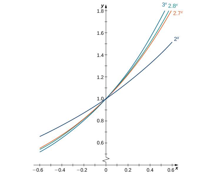
We make one final assumption: that there is a unique value of \(b>0\) for which \(B′(0)=1\). We define e to be this unique value, as we did in Introduction to Functions and Graphs. Figure \(\PageIndex{1}\) provides graphs of the functions \(y=2^x, \,y=3^x, \,y=2.7^x,\) and \(y=2.8^x\). A visual estimate of the slopes of the tangent lines to these functions at 0 provides evidence that the value of e lies somewhere between 2.7 and 2.8. The function \(E(x)=e^x\) is called the natural exponential function. Its inverse, \(L(x)=\log_e (x)=\ln (x)\) is called the natural logarithmic function.

Figure \(\PageIndex{2}\): The graph of \(E(x)=e^x\) is between \(y=2^x\) and \(y=3^x\).

For a better estimate of \(e\), we may construct a table of estimates of \(B′(0)\) for functions of the form \(B(x)=b^x\). Before doing this, recall that

\[B′(0)=\lim_{x→0}\dfrac{b^x−b^0}{x−0}=\lim_{x→0}\dfrac{b^x−1}{x}≈\dfrac{b^x−1}{x} \nonumber \]

for values of \(x\) very close to zero. If we choose \(x=0.00001\) and \(x=−0.00001\) to obtain the estimate, this gives:

\[\dfrac{b^{−0.00001}−1}{−0.00001}<B′(0)< \dfrac{b^{0.00001}−1}{0.00001} \nonumber \]

See the following table.

Table : Estimating the value of \(e\)

\(b\)	\(\dfrac{b^{−0.00001}−1}{−0.00001}<B′(0)<\dfrac{b^{0.00001}−1}{0.00001}\)	\(b\)	\(\dfrac{b^{−0.00001}−1}{−0.00001}<B′(0)<\dfrac{b^{0.00001}−1}{0.00001}\)
2	\(0.693145<B′(0)<0.69315\)	2.7183	\(1.000002<B′(0)<1.000012\)
2.7	\(0.993247<B′(0)<0.993257\)	2.719	\(1.000259<B′(0)<1.000269\)
2.71	\(0.996944<B′(0)<0.996954\)	2.72	\(1.000627<B′(0)<1.000637\)
2.718	\(0.999891<B′(0)<0.999901\)	2.8	\(1.029614<B′(0)<1.029625\)
2.7182	\(0.999965<B′(0)<0.999975\)	3	\(1.098606<B′(0)<1.098618\)

The evidence from the table suggests that since \(2.7182^x<e^x<2.7183^x\), the function \(E(x)=e^x\) we will have \(0.999965<E'(0)<1.000012\), so \(E'(0)\approx 1\).

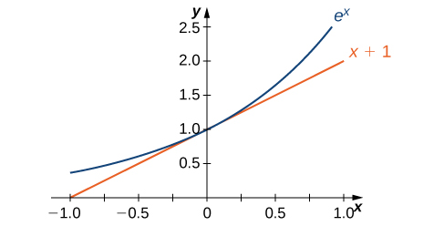
The graph of \(E(x)=e^x\) together with the line \(y=x+1\) are shown in Figure \(\PageIndex{2}\). This line is tangent to the graph of \(E(x)=e^x\) at \(x=0\).

Figure \(\PageIndex{2}\): The tangent line to \(E(x)=e^x\) at \(x=0\) has slope 1.

Now that we have laid out our basic assumptions, we begin our investigation by exploring the derivative of \(B(x)=b^x, \,b>0\).
Recall that we have assumed that \(B′(0)\) exists. By applying the limit definition to the derivative we conclude that

\[B′(0)=\lim_{h→0}\frac{b^{0+h}−b^0}{h}=\lim_{h→0}\frac{b^h−1}{h} \nonumber \]

Turning to \(B′(x)\), we obtain the following.

\[\begin{align*} \displaystyle B′(x)&=\lim_{h→0}\frac{b^{x+h}−b^x}{h} & & \text{Apply the limit definition of the derivative.}\\[4pt]
&=\lim_{h→0}\frac{b^xb^h−b^x}{h} & & \text{Note that }b^{x+h}=b^xb^h.\\[4pt]
&=\lim_{h→0}\frac{b^x(b^h−1)}{h} & & \text{Factor out }b^x.\\[4pt]
&=b^x\lim_{h→0}\frac{b^h−1}{h} & & \text{Apply a property of limits.}\\[4pt]
&=b^xB′(0) & & \text{Use } B′(0)=\lim_{h→0}\frac{b^{0+h}−b^0}{h}=\lim_{h→0}\frac{b^h−1}{h}.\end{align*}\]

We see that on the basis of the assumption that \(B(x)=b^x\) is differentiable at \(0,B(x)\) is not only differentiable everywhere, but its derivative is

\[B′(x)=b^xB′(0) \nonumber \]

For \(E(x)=e^x, \,E′(0)=1.\) Thus, we have \(E′(x)=e^x\). (The value of \(B′(0)\) for an arbitrary function of the form \(B(x)=b^x, \,b>0,\) will be derived later.)

Derivative of the Natural Exponential Function

Let \(f(x)=e^x\) be the natural exponential function. Then

\[f′(x)=e^x \nonumber \]

 

Example \(\PageIndex{7}\)

Find the equation of the line tangent to \(y=3e^x-2x^2+4x\) at the point where \(x=1\).

Solution

To find the tangent line at this point, we need the height and slope of the function \(f(x)=3e^x-2x^2+4x\) at \(x=1\).

Plugging in \(x=1\) into this function gives \(f(1)=3e^1-2\cdot 1^2+4\cdot 1=3e+2\). Thus, the tangent point is \(\left(1,3e+2\right)\).

In order to find the slope at this point, we take the derivative of \(f(x)\):

\[ \begin{align*} f'(x)&=\dfrac{d}{dx}\left( 3e^x-2x^2+4x\right) \\ &= \dfrac{d}{dx}\left(3e^x\right)-\dfrac{d}{dx}\left(2x^2\right)+\dfrac{d}{dx}\left(4x\right) \\ &= 3\dfrac{d}{dx}\left(e^x\right)-2\dfrac{d}{dx}\left(x^2\right)+4 \\ &= 3\cdot  e^x -2\cdot 2x+4 \\ &=3e^x-4x+4 \end{align*} \]

Plugging in \(x=1\) into \(f'(x)\) gives \(f'(1)=3e^1-4\cdot 1+4= 3e\). This is the slope of our tangent line. 

Therefore, since the tangent line we are looking for is \(y-f(1)=f'(1)(x-1)\), we have \(y-(3e+2)=3e\cdot (x-1)\).

Putting this into slope-intercept form, we get our final answer: \(\boxed{y=3e x+2}\).

Exercise \(\PageIndex{6}\)

Find the equation of the line tangent to \(y=e^{7+x}-1\) at the point where \(x=-7\).

Hint

Write \(e^{7+x}\) as \(e^7\cdot e^x\), and recall that \(e^7\) is a constant. Follow the steps in Example \(\PageIndex{7}\).

Answer

\(y=x+7\)

Key Concepts

• The derivative of a constant function is zero.
• The derivative of a power function is a function in which the power on \(x\) becomes the coefficient of the term and the power on \(x\) in the derivative decreases by 1.
• The derivative of a constant \(c\) multiplied by a function \(f\) is the same as the constant multiplied by the derivative.
• The derivative of the sum of a function \(f\) and a function \(g\) is the same as the sum of the derivative of \(f\) and the derivative of \(g\).
• The derivative of the difference of a function \(f\) and a function \(g\) is the same as the difference of the derivative of \(f\) and the derivative of \(g\).

Key Equations

• Derivative of the constant function

\(\dfrac{d}{dx}\Big(C\Big)=0\)

• Derivative of the linear function

\(\dfrac{d}{dx}\Big(mx+b\Big)=m\)

• Derivative of the power function

\(\dfrac{d}{dx}\Big(x^n\Big)=nx^{n-1}\)

Glossary

constant multiple rule

the derivative of a constant \(c\) multiplied by a function \(f\) is the same as the constant multiplied by the derivative: \(\dfrac{d}{dx}\big(cf(x)\big)=cf′(x

difference rule

the derivative of the difference of a function \(f\) and a function \(g\) is the same as the difference of the derivative of \(f\) and the derivative of \(g\): \(\dfrac{d}{dx}\left(f(x)-g(x)\right)=f′(x)-g′(x)\)

power rule

the derivative of a power function is a function in which the power on \(x\) becomes the coefficient of the term and the power on \(x\) in the derivative decreases by 1: If \(n\) is an integer, then \(\dfrac{d}{dx}\left(x^n\right)=nx^{n−1}\)

sum rule

the derivative of the sum of a function \(f\) and a function \(g\) is the same as the sum of the derivative of \(f\) and the derivative of \(g\): \(\dfrac{d}{dx}\left(f(x)+g(x)\right)=f′(x)+g′(x)\)