3.11: Hyperbolic Functions

Learning Objectives

• Identify the hyperbolic functions, their graphs, and basic identities.
• Apply the formulas for derivatives of the hyperbolic functions and their inverses.
• Describe the common applied conditions of a catenary curve.

Hyperbolic Functions

The hyperbolic functions are defined in terms of certain combinations of \(e^x\) and \(e^{−x}\). These functions arise naturally in various engineering and physics applications, including the study of water waves and vibrations of elastic membranes. Another common use for a hyperbolic function is the representation of a hanging chain or cable, also known as a catenary (Figure \(\PageIndex{1}\)). If we introduce a coordinate system so that the low point of the chain lies along the \(y\)-axis, we can describe the height of the chain in terms of a hyperbolic function. First, we define the hyperbolic functions.

Figure \(\PageIndex{1}\):The shape of a strand of silk in a spider’s web can be described in terms of a hyperbolic function. The same shape applies to a chain or cable hanging from two supports with only its own weight. (credit: “Mtpaley”, Wikimedia Commons)

Definitions: Hyperbolic Functions

Hyperbolic cosine

\(\cosh (x)=\dfrac{e^x+e^{−x}}{2}\)

Hyperbolic sine

\(\sinh (x)=\dfrac{e^x−e^{−x}}{2}\)

Hyperbolic tangent

\(\tanh (x)=\dfrac{\sinh (x)}{\cosh (x)}=\dfrac{e^x−e^{−x}}{e^x+e^{−x}}\)

Hyperbolic cosecant

\(\operatorname{csch}(x)=\dfrac{1}{\sinh (x)}=\dfrac{2}{e^x−e^{−x}}\)

Hyperbolic secant

\(\operatorname{sech}(x)=\dfrac{1}{\cosh (x)}=\dfrac{2}{e^x+e^{−x}}\)

Hyperbolic cotangent

\(\coth (x)=\dfrac{\cosh (x)}{\sinh (x)}=\dfrac{e^x+e^{−x}}{e^x−e^{−x}}\)

The name \(\cosh\) rhymes with “gosh,” whereas the name \(\sinh\) is pronounced “cinch.” \(\operatorname{tanh}, \,\operatorname{sech}, \, \operatorname{csch},\) and \(\coth\) are pronounced “tanch,” “seech,” “coseech,” and “cotanch,” respectively.

Using the definition of \(\cosh(x)\) and principles of physics, it can be shown that the height of a hanging chain, such as the one in Figure \(\PageIndex{7}\), can be described by the function \(h(x)=a\cosh\left(\dfrac{x}{a}\right) + c\) for certain constants \(a\) and \(c\).

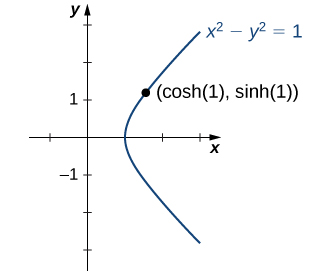
But why are these functions called hyperbolic functions? To answer this question, consider the quantity \(\cosh^2 (t) − \sinh^2 (t)\). Using the definition of \(\cosh\) and \(\sinh\), we see that

\[\cosh^2 (t) − \sinh^2 (t)=\dfrac{e^{2t}+2+e^{−2t}}{4}−\dfrac{e^{2t}−2+e^{−2t}}{4}=1 \nonumber \]

This identity is the analog of the trigonometric identity \(\cos^2 (t) + \sin^2 (t)=1\) that we have seen for our circular trigonmetric functions. Here, given a value \(t\), the point \((x,y)=\left(\cosh (t),\,\sinh (t)\right)\) lies on the unit hyperbola \(x^2−y^2=1\) (Figure \(\PageIndex{2}\)) instead of the unit circle.

Figure \(\PageIndex{2}\): The unit hyperbola \(\cosh^2 (t) − \sinh^2 (t)=1\).

Graphs of Hyperbolic Functions

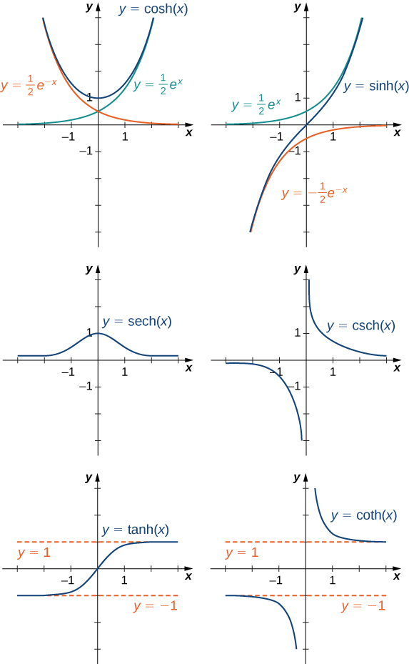
To graph \(\cosh (x)\) and \(\sinh (x)\), we make use of the fact that both functions approach \(\dfrac{1}{2}e^x\) as \(x→∞\), since \(e^{−x}→0\) as \(x→∞\). As \(x→−∞,\cosh (x)\) approaches \(\dfrac{1}{2}e^{−x}\), whereas \(\sinh (x)\) approaches \(-\dfrac{1}{2}e^{−x}\). Therefore, using the graphs of \(\dfrac{1}{2}e^x,\dfrac{1}{2}e^{−x}\), and \(-\dfrac{1}{2}e^{−x}\) as guides, we graph \(\cosh (x)\) and \(\sinh (x)\).

To graph \(\tanh (x)\), we use the fact that \(\tanh(0)=0\), \(−1<\tanh(x)<1\) for all \(x\), \(\tanh (x)→1\) as \(x→∞\), and \(\tanh (x)→−1\) as \(x→−∞\). The graphs of the other three hyperbolic functions can be sketched using the graphs of \(\cosh (x)\), \(\sinh (x)\), and \(\tanh (x)\) (Figure \(\PageIndex{3}\)) and considering their reciprocal values.

Figure \(\PageIndex{3}\): The hyperbolic functions involve combinations of \(e^x\) and \(e^{−x}\).

Identities Involving Hyperbolic Functions

The identity \(\cosh^2 (t)−\sinh^2 (t) = 1\), shown in Figure \(\PageIndex{8}\), is one of several identities involving the hyperbolic functions, some of which are listed next. The first four properties follow easily from the definitions of hyperbolic sine and hyperbolic cosine. Except for some differences in signs, most of these properties are analogous to identities for trigonometric functions.

Identities Involving Hyperbolic Functions

1. \(\cosh(−x)=\cosh (x)\)
2. \(\sinh(−x)=−\sinh (x)\)
3. \(\cosh (x)+\sinh (x)=e^x\)
4. \(\cosh (x)−\sinh (x)=e^{−x}\)
5. \(\cosh^2 (x)−\sinh^2 (x)=1\)
6. \(1−\tanh^2 (x)=\operatorname{sech}^2 (x)\)
7. \(\coth^2 (x) −1=\operatorname{csch}^2 (x)\)
8. \(\sinh(x±y)=\sinh (x) \cosh (y) ± \cosh (x) \sinh (y)\)
9. \(\cosh(x±y)=\cosh (x) \cosh (y) ± \sinh (x) \sinh (y)\)

Example \(\PageIndex{1}\): Evaluating Hyperbolic Functions

1. Simplify \(\sinh\left(5\ln (x)\right)\)
2. If \(\sinh (x)=\dfrac{3}{4}\), find the values of the remaining five hyperbolic functions.

Solution:

a. Using the definition of the \(\sinh\) function, we write \(\sinh\left(5\ln (x)\right)=\dfrac{e^{5\ln (x)}−e^{−5\ln (x)}}{2}=\dfrac{e^{\ln (x^5)}−e^{\ln (x^{−5})}}{2}=\boxed{\dfrac{x^5−x^{−5}}{2}}\)

b. Using the identity \(\cosh^2 (x) − \sinh^2 (x)=1\), we see that \(\cosh^2 (x)=1+\left(\dfrac{3}{4}\right)^2=\dfrac{25}{16}\).

Since \(\cosh (x)≥1\) for all \(x\), we must have \(\boxed{\cosh (x)=\dfrac{5}{4}}\).

Then, using the definitions for the other hyperbolic functions, we conclude that:

\(\boxed{\tanh (x)=\dfrac{3}{5},\, \operatorname{csch}(x)=\dfrac{4}{3},\,\operatorname{sech}(x)=\dfrac{4}{5},\, \text{ and } \coth (x)=\dfrac{5}{3}}\)

Exercise \(\PageIndex{1}\)

Simplify \(\cosh\left(2\ln (x)\right)\)

Hint

Use the definition of the \(\cosh\) function and the power property of logarithm functions.

Answer

\(\dfrac{x^2+x^{−2}}{2}\)

Inverse Hyperbolic Functions

From the graphs of the hyperbolic functions, we see that all of them are one-to-one except \(\cosh x\) and \(\operatorname{sech}x\). If we restrict the domains of these two functions to the interval \([0,∞),\) then all the hyperbolic functions are one-to-one, and we can define the inverse hyperbolic functions. Since the hyperbolic functions themselves involve exponential functions, the inverse hyperbolic functions involve logarithmic functions.

Definitions: Inverse Hyperbolic Functions

\[\begin{align*} &\sinh^{−1} (x) =\operatorname{arcsinh} (x) =\ln \left(x+\sqrt{x^2+1}\right) & & \cosh^{−1} (x) =\operatorname{arccosh} (x) =\ln \left(x+\sqrt{x^2−1}\right)\\[4pt]
&\tanh^{−1} (x) =\operatorname{arctanh} (x) =\dfrac{1}{2}\ln \left(\dfrac{1+x}{1−x}\right) & & \coth^{−1} (x) =\operatorname{arccot} (x) =\frac{1}{2}\ln \left(\dfrac{x+1}{x−1}\right)\\[4pt]
&\operatorname{sech}^{−1} (x) =\operatorname{arcsech} (x) =\ln \left(\dfrac{1+\sqrt{1−x^2}}{x}\right) & & \operatorname{csch}^{−1} (x) =\operatorname{arccsch} (x) =\ln \left(\dfrac{1}{x}+\dfrac{\sqrt{1+x^2}}{|x|}\right) \end{align*}\]

Let’s look at how to derive the first equation. The others follow similarly. Suppose \(y=\sinh^{−1} (x) \). Then, \(x=\sinh (y) \) and, by the definition of the hyperbolic sine function, \(x=\dfrac{e^y−e^{−y}}{2}\). Therefore,

\(e^y−2x−e^{−y}=0\)

Multiplying this equation by \(e^y\), we obtain

\(e^{2y}−2xe^y−1=0\)

This can be solved like a quadratic equation, with the solution

\(e^y=\dfrac{2x±\sqrt{4x^2+4}}{2}=x±\sqrt{x^2+1}\)

Since \(e^y>0\),the only solution is the one with the positive sign. Applying the natural logarithm to both sides of the equation, we conclude that

\(y=\ln (x+\sqrt{x^2+1})\)

This gives the formula for \(\sinh^{-1}(x)\) we see above. The other five inverses are derived similarly.

Example \(\PageIndex{2}\): Evaluating Inverse Hyperbolic Functions

Evaluate each of the following expressions.

a. \(\sinh^{−1}(2)\)

b. \(\tanh^{−1}\left(\dfrac{1}{4}\right)\)

Solution:

a. \[\sinh^{−1}(2)=\ln (2+\sqrt{2^2+1})=\boxed{\ln (2+\sqrt{5})≈1.4436} \nonumber \]

b. \[\tanh^{−1}\left(\dfrac{1}{4}\right)=\frac{1}{2}\ln \left(\dfrac{1+\frac{1}{4}}{1−\frac{1}{4}}\right)=\frac{1}{2}\ln \left(\dfrac{\frac{5}{4}}{\frac{3}{4}}\right)=\boxed{\frac{1}{2}\ln \left(\dfrac{5}{3}\right)≈0.2554}\nonumber \]

Exercise \(\PageIndex{2}\)

Evaluate \(\tanh^{−1}\left(\dfrac{1}{2}\right)\).

Hint

Use the definition of \(\tanh^{−1}(x)\) and simplify.

Answer

\(\dfrac{1}{2}\ln (3)≈0.5493\)

Derivatives of Hyperbolic Functions

It is easy to develop differentiation formulas for the hyperbolic functions. For example, looking at \(\sinh (x)\) we have

\[\begin{align*} \dfrac{d}{dx} \left(\sinh (x) \right) &=\dfrac{d}{dx} \left(\dfrac{e^x−e^{−x}}{2}\right) \\[4pt] &=\dfrac{1}{2}\left[\dfrac{d}{dx}\left(e^x\right)−\dfrac{d}{dx}\left(e^{−x}\right)\right] \\[4pt] &=\dfrac{1}{2}\left[e^x+e^{−x}\right] \\[4pt] &=\cosh (x) \end{align*} \nonumber \]

Similarly,

\[\dfrac{d}{dx} \cosh (x)=\sinh (x) \nonumber \]

We summarize the differentiation formulas for the hyperbolic functions in Table \(\PageIndex{1}\).

Table \(\PageIndex{1}\): Derivatives of the Hyperbolic Functions

\(f(x)\)	\(\dfrac{d}{dx}f(x)\)
\(\sinh (x)\)	\(\cosh (x)\)
\(\cosh (x)\)	\(\sinh (x)\)
\(\tanh (x)\)	\(\text{sech}^2 \,(x)\)
\(\text{coth } (x)\)	\(−\text{csch}^2\, (x)\)
\(\text{sech } (x)\)	\(−\text{sech}\, (x) \tanh (x)\)
\(\text{csch } (x)\)	\(−\text{csch}\, (x) \coth (x)\)

Let’s take a moment to compare the derivatives of the hyperbolic functions with the derivatives of the standard trigonometric functions. There are a lot of similarities, but differences as well. For example, the derivatives of the sine functions match:

\[\dfrac{d}{dx} \sin (x)=\cos (x) \quad \text{and} \quad  \dfrac{d}{dx} \sinh(x)=\cosh (x) \nonumber \]

The derivatives of the cosine functions, however, differ in sign:

\[\dfrac{d}{dx} \cos (x)=−\sin(x) \quad \text{but} \quad  \dfrac{d}{dx} \cosh (x)=\sinh (x)\nonumber \]

Example \(\PageIndex{3}\): Differentiating Hyperbolic Functions

Evaluate the following derivatives:

1. \(\dfrac{d}{dx}\left[\sinh\left(x^2\right)\right]\)
2. \(\dfrac{d}{dx}\left[\cosh^2 (x)\right]\)

Solution:

Using the formulas in Table \(\PageIndex{1}\) and the chain rule, we get

(a) \(\boxed{\dfrac{d}{dx}\left[\sinh\left(x^2\right)\right]=\cosh\left(x^2\right)⋅2x}\)

(b) \(\boxed{\dfrac{d}{dx}\left[\cosh^2 (x)\right]=2\cosh (x)\cdot \sinh (x)}\)

Exercise \(\PageIndex{3}\)

Evaluate the following derivatives:

1. \(\dfrac{d}{dx}\left[\tanh\left(x^2+3x\right)\right]\)
2. \(\dfrac{d}{dx}\left[\dfrac{1}{\sinh^3 (x)}\right]\)

Hint

Use the formulas in Table \(\PageIndex{1}\) and apply the chain rule as necessary.

Answer a

\(\dfrac{d}{dx}\left[\tanh\left(x^2+3x\right)\right]=\text{sech}^2\left(x^2+3x\right)\cdot (2x+3)\)

Answer b

\(\dfrac{d}{dx}\left[\dfrac{1}{\sinh^3 (x)}\right]=\dfrac{d}{dx}\left[( \left(\sinh (x)\right)^{−3}\right]=−3\left(\sinh (x)\right)^{−4}\cdot \cosh (x)\)

Just like we did for the inverse trigonometric functions, we can use the inverse derivative formula to differentiate these inverse hyperbolic functions.

If \(f(x)=\sinh(x)\) has \(f'(x)=\cosh(x)\), and we want the derivative of \(f^{-1}(x)=\sinh^{-1}(x)\), we have:

\[   \dfrac{d}{dx}\left(f^{-1}(x)\right)=\dfrac{1}{f'\left(f^{-1}(x)\right)}=\dfrac{1}{\cosh\left(\sinh^{-1}(x)\right)} \nonumber \]

We can evaluate this composition:

\[\cosh\left(\sinh^{-1}(x)\right)=\dfrac{e^{\ln\left(x+\sqrt{x^2+1}\right)}+e^{-\ln\left(x+\sqrt{x^2+1}\right)}}{2}=\dfrac{x+\sqrt{x^2+1}+\frac{1}{x+\sqrt{x^2+1}}}{2}=\dfrac{1}{\sqrt{x^2+1}} \nonumber \]

Thus,

\[\dfrac{d}{dx} \left( \sinh^{-1} (x)\right)=\dfrac{1}{\sqrt{x^2+1}} \nonumber \]

We summarize the differentiation formulas for the remaining inverse hyperbolic functions in Table \(\PageIndex{2}\).

Table \(\PageIndex{2}\): Derivatives of the Inverse Hyperbolic Functions

\(f(x)\)	\(\dfrac{d}{dx}f(x)\)
\(\sinh^{-1} (x)\)	\(\dfrac{1}{\sqrt{x^2+1}}\)
\(\cosh^{-1} (x)\)	\(\dfrac{1}{\sqrt{x^2-1}}\) for \(|x|>1\)
\(\tanh^{-1} (x)\)	\(\dfrac{1}{1-x^2}\) for \(|x|<1\)
\(\text{coth}^{-1} (x)\)	\(\dfrac{1}{1-x^2}\) for \(|x|>1\)
\(\text{sech}^{-1} (x)\)	\(-\dfrac{1}{x\sqrt{1-x^2}}\) for \(0<x<1\)
\(\text{csch}^{-1} (x)\)	\(-\dfrac{1}{x\sqrt{1+x^2}}\) for \(x>0\)

Example \(\PageIndex{4}\): Differentiating Inverse Hyperbolic Functions

Find the equation of the line tangent to \(y=4x\left(1+\text{sech}^{-1}\left(\sqrt{x}\right)\right)\) when \(x=\dfrac{3}{4}\)

Solution:

First, we need to find the height of our function at \(x=\dfrac{3}{4}\):

\[y=4\cdot \dfrac{3}{4}\left(1+\text{sech}^{-1}\left( \sqrt{\dfrac{3}{4}}\right)\right)= 3\left(1+\text{sech}^{-1}\left(\dfrac{\sqrt{3}}{2}\right)\right) \nonumber \]

Note that \(\text{sech}^{-1}\left( \dfrac{\sqrt{3}}{2}\right)= \ln\left( \dfrac{1+\sqrt{1-\left(\frac{\sqrt{3}}{2}\right)^2}}{\frac{\sqrt{3}}{2}}\right)=\ln\left(\sqrt{3}\right)=\dfrac{1}{2}\ln(3)\), so we go through the point \(\left(\dfrac{3}{4},3+\dfrac{3}{2}\ln(3)\right)\).

Next, we need to find the slope of the tangent line, so we take the derivative using the formulas in Table \(\PageIndex{2}\) and the product chain rule:

\[  \dfrac{dy}{dx}=4\left(1+\text{sech}^{-1}\left(\sqrt{x}\right)\right)+4x\cdot \left(- \dfrac{1}{\sqrt{x}\cdot \sqrt{1-\left(\sqrt{x}\right)^2}}\cdot \dfrac{1}{2}x^{-\frac{1}{2}}\right)=4+4\text{sech}^{-1}\left(\sqrt{x}\right)-\dfrac{2}{\sqrt{1-x}}  \nonumber \]

Plugging in \(x=\dfrac{3}{4}\), we get:

\[y'\left(\dfrac{3}{4}\right)=4+4\text{sech}^{-1}\left( \dfrac{\sqrt{3}}{2}\right)-\dfrac{2}{\sqrt{1-\frac{3}{4}}}=4+4\cdot \dfrac{1}{2}\ln(3)-4=2\ln(3) \nonumber\]

Therefore, our tangent line must be \(y=2\ln(3)\cdot \left( x-\dfrac{3}{4}\right)+\left(3+\dfrac{3}{2}\ln(3)\right)\). This simplifies to

\[\boxed{ y=2\ln(3)\cdot x +3}\nonumber \]

Exercise \(\PageIndex{4}\)

Find the equation of the line tangent to \(y=3x\sinh^{-1}(x)-3\sqrt{x^2+1}\) at the point where \(x=\dfrac{4}{3}\)

Hint

Follow the steps in Example \(\PageIndex{4}\) above.

Answer

\(y=3\ln(3)\cdot x -5\)

Applications

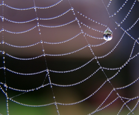
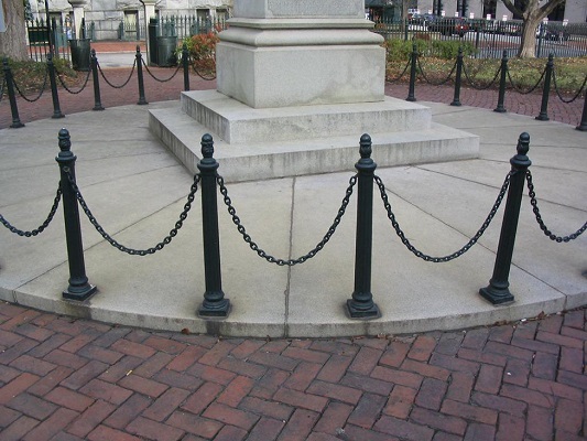
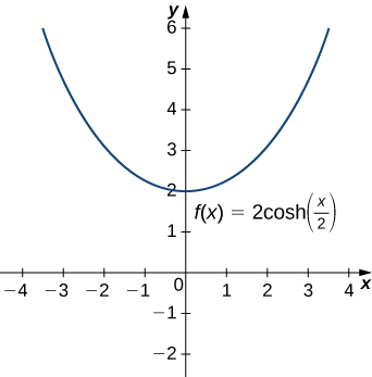
One physical application of hyperbolic functions involves hanging cables. If a cable of uniform density is suspended between two supports without any load other than its own weight, the cable forms a curve called a catenary. High-voltage power lines, chains hanging between two posts, and strands of a spider’s web all form catenaries. The following figure shows chains hanging from a row of posts.

Figure \(\PageIndex{4}\): Chains between these posts take the shape of a catenary. (credit: modification of work by OKFoundryCompany, Flickr)

Hyperbolic functions can be used to model catenaries. Specifically, functions of the form \(y=a\cdot \cosh\left(\dfrac{x}{a}\right)\) are catenaries. Figure \(\PageIndex{5}\) shows the graph of \(y=2\cosh\left(\dfrac{x}{2}\right)\).

Figure \(\PageIndex{5}\): A hyperbolic cosine function forms the shape of a catenary.

Key Concepts

• Hyperbolic functions are defined in terms of exponential functions.
• Term-by-term differentiation yields differentiation formulas for the hyperbolic functions. These differentiation formulas give rise, in turn, to integration formulas.
• With appropriate range restrictions, the hyperbolic functions all have inverses involving the natural logarithm.
• Implicit differentiation yields differentiation formulas for the inverse hyperbolic functions.
• The most common physical applications of hyperbolic functions are calculations involving catenaries.

Key Equations

• Derivative of the hyperbolic sine function

\(\dfrac{d}{dx}\left(\sinh (x)\right)=\cosh(x)\)

• Derivative of the hyperbolic cosine function

\(\dfrac{d}{dx}\left(\cosh (x)\right)=\sinh(x)\)

• Derivative of the hyperbolic tangent function

\(\dfrac{d}{dx}\left(\tanh (x)\right)=\text{sech}^2 (x) \)

• Derivative of the hyperbolic cotangent function

\(\dfrac{d}{dx}\left(\text{coth} (x)\right)=−\text{csch}^2 (x) \)

• Derivative of the hyperbolic secant function

\(\dfrac{d}{dx}\left(\text{sech} (x)\right)=-\text{sech}(x)\tanh(x)\)

• Derivative of the hyperbolic cosecant function

\(\dfrac{d}{dx}\left(\text{csch} (x)\right)=−\text{csch}(x)\text{coth}(x)\)

• Derivative of the inverse hyperbolic sine function

\(\dfrac{d}{dx}\left(\sinh^{-1} (x)\right)=\dfrac{1}{\sqrt{x^2+1}} \)

• Derivative of the inverse hyperbolic cosine function

\(\dfrac{d}{dx}\left(\cosh^{-1} (x)\right)=\dfrac{1}{\sqrt{x^2-1}} \)

• Derivative of the inverse hyperbolic tangent function

\(\dfrac{d}{dx}\left(\tanh^{-1} (x)\right)=\dfrac{1}{1-x^2}\)

• Derivative of the inverse hyperbolic cotangent function

\(\dfrac{d}{dx}\left(\text{coth}^{-1} (x)\right)=\dfrac{1}{1-x^2}\)

• Derivative of the inverse hyperbolic secant function

\(\dfrac{d}{dx}\left(\text{sech}^{-1} (x)\right)=-\dfrac{1}{x\sqrt{1-x^2}} \)

• Derivative of the inverse hyperbolic cosecant function

\(\dfrac{d}{dx}\left(\text{csch}^{-1} (x)\right)=−\dfrac{1}{x\sqrt{1+x^2}} \)

Glossary

catenary

a curve in the shape of the function \(y=a\cdot\cosh\left(\dfrac{x}{a}\right)\) is a catenary; a cable of uniform density suspended between two supports assumes the shape of a catenary

hyperbolic functions

the functions denoted \(\sinh,\,\cosh,\,\operatorname{tanh},\,\operatorname{csch},\,\operatorname{sech},\) and \(\coth\), which involve certain combinations of \(e^x\) and \(e^{−x}\)

inverse hyperbolic functions

the inverses of the hyperbolic functions where \(\cosh\) and \( \operatorname{sech}\) are restricted to the domain \([0,∞)\); each of these functions can be expressed in terms of a composition of the natural logarithm function and an algebraic function