5.1: Antiderivatives

At this point, we have seen how to calculate derivatives of many functions and have been introduced to a variety of their applications. We now ask a question that turns this process around: Given a function \(f\), how do we find a function with the derivative \(f\) and why would we be interested in such a function?

We answer the first part of this question by defining anti-derivatives. The anti-derivative of a function \(f\) is a function with a derivative \(f\). Why are we interested in anti-derivatives? The need for anti-derivatives arises in many situations, and we look at various examples throughout the remainder of the text. Here we examine one specific example that involves rectilinear motion. In our examination in Derivatives of rectilinear motion, we showed that given a position function \(s(t)\) of an object, then its velocity function \(v(t)\) is the derivative of \(s(t)\)—that is, \(v(t)=s′(t)\). Furthermore, the acceleration \(a(t)\) is the derivative of the velocity \(v(t)\)—that is, \(a(t)=v′(t)=s''(t)\). Now suppose we are given an acceleration function \(a\), but not the velocity function v or the position function \(s\). Since \(a(t)=v′(t)\), determining the velocity function requires us to find an anti-derivative of the acceleration function. Then, since \(v(t)=s′(t),\) determining the position function requires us to find an anti-derivative of the velocity function. Rectilinear motion is just one case in which the need for anti-derivatives arises. We will see many more examples throughout the remainder of the text. For now, let’s look at the terminology and notation for anti-derivatives, and determine the anti-derivatives for several types of functions. We examine various techniques for finding anti-derivatives of more complicated functions later in the text (Introduction to Techniques of Integration).

The Reverse of Differentiation

At this point, we know how to find derivatives of various functions. We now ask the opposite question. Given a function \(f\), how can we find a function with derivative \(f\)? If we can find a function \(F\) derivative \(f,\) we call \(F\) an anti-derivative of \(f\).

Definition: Anti-derivative

A function \(F\) is an anti-derivative of the function \(f\) if

\[F′(x)=f(x) \nonumber \]

for all \(x\) in the domain of \(f\).

Consider the function \(f(x)=2x\). Knowing the power rule of differentiation, we conclude that \(F(x)=x^2\) is an anti-derivative of \(f\) since \(F′(x)=2x\). Are there any other anti-derivatives of \(f\)? Yes; since the derivative of any constant \(C\) is zero, \(x^2+C\) is also an anti-derivative of \(2x\). Therefore, \(x^2+5\) and \(x^2-\sqrt{2}\) are also anti-derivatives. Are there any others that are not of the form \(x^2+C\) for some constant \(C\)? The answer is no. From Corollary 2 of the Mean Value Theorem, we know that if \(F\) and \(G\) are differentiable functions such that \(F′(x)=G′(x),\) then \(F(x)-G(x)=C\) for some constant \(C\). This fact leads to the following important theorem.

Theorem \(\PageIndex{1}\): General Form of an Anti-derivative 

Let \(F\) be an anti-derivative of \(f\) over an interval \(I\). Then,

1. for each constant \(C\), the function \(F(x)+C\) is also an anti-derivative of \(f\) over \(I\);
2. if \(G\) is an anti-derivative of \(f\) over \(I\), there is a constant \(C\) for which \(G(x)=F(x)+C\) over \(I\).

In other words, the most general form of the anti-derivative of \(f\) over \(I\) is \(F(x)+C\).

We use this fact and our knowledge of derivatives to find all the anti-derivatives for several functions.

Example \(\PageIndex{1}\): Finding Anti-derivatives

For each of the following functions, find all anti-derivatives.

1. \(f(x)=3x^2\)
2. \(f(x)=\dfrac{1}{x}\)
3. \(f(x)=\cos (x)\)
4. \(f(x)=e^x\)

Solution

(a) Because

\[\dfrac{d}{dx}\left(x^3\right)=3x^2 \nonumber\]

then \(F(x)=x^3\) is an anti-derivative of \(3x^2\). Therefore, every anti-derivative of \(3x^2\) is of the form \(x^3+C\) for some constant \(C\), and every function of the form \(\boxed{x^3+C}\) is an anti-derivative of \(3x^2\).

(b) Let \(f(x)=\ln |x|.\) For \(x>0,f(x)=\ln (x)\) and

\[\dfrac{d}{dx}\left(\ln(x)\right)=\dfrac{1}{x} \nonumber\]

For \( x<0,f(x)=\ln (−x)\) and

\[\dfrac{d}{dx}\left(\ln (−x)\right)=−\dfrac{1}{−x}=\dfrac{1}{x} \nonumber\]

Therefore,

\[\dfrac{d}{dx}\left(\ln |x|\right)=\dfrac{1}{x} \nonumber\]

Thus, \(F(x)=\ln |x|\) is an anti-derivative of \(\dfrac{1}{x}\). Therefore, every anti-derivative of \(\dfrac{1}{x}\) is of the form \(\ln |x|+C\) for some constant \(C\) and every function of the form \(\boxed{\ln |x|+C}\) is an anti-derivative of \(\dfrac{1}{x}\).

(c) We have

\[\dfrac{d}{dx}\left(\sin (x)\right)=\cos(x)\nonumber\]

so \(F(x)=\sin(x)\) is an anti-derivative of \(\cos (x)\). Therefore, every anti-derivative of \(\cos (x)\) is of the form \(\sin (x)+C\) for some constant \(C\) and every function of the form \(\boxed{\sin (x)+C}\) is an anti-derivative of \(\cos(x)\).

(d) Since

\[\dfrac{d}{dx}\left(e^x\right)=e^x \nonumber\]

then \(F(x)=e^x\) is an anti-derivative of \(e^x\). Therefore, every anti-derivative of \(e^x\) is of the form \(e^x+C\) for some constant \(C\) and every function of the form \(\boxed{e^x+C}\) is an anti-derivative of \(e^x\).

Exercise \(\PageIndex{1}\)

Find all anti-derivatives of \(f(x)=\sin (x)\)

Answer

\(−\cos (x)+C\)

Anti-derivative Shortcuts

We can see that all of our previous knowledge about derivatives has an equivalent statement about anti-derivatives.

Table : Anti-derivative Shortcut Formulas

\(f(x)=F'(x)\)	\(F(x)\)
\(0\)	\(C\)
\(k\) (a constant function)	\(kx+C\)
\(x^n\) for \(n\ne -1\)	\(\dfrac{1}{n+1}x^{n+1}+C\)
\(\dfrac{1}{x}\)	\(\ln |x|+C\)
\(e^x\)	\(e^x+C\)
\(b^x\)	\(\dfrac{1}{\ln(b)}b^x+C\)
\(\cos (x)\)	\(\sin (x)+C\)
\(\sin (x)\)	\(-\cos (x)+C\)
\(\sec^2(x)\)	\(\tan (x)+C\)
\(\csc^2(x)\)	\(-\cot (x)+C\)
\(\sec(x)\tan (x)\)	\(\sec(x)+C\)
\(\csc(x)\cot (x)\)	\(-\csc(x)+C\)
\(\dfrac{1}{\sqrt{1−x^2}}\)	\(\sin^{-1}(x)+C\)
\(\dfrac{1}{1+x^2}\)	\(\tan^{-1}(x)+C\)
\(\dfrac{1}{x\sqrt{x^2−1}}\)	\(\sec^{-1}(x)+C\)

Similarly, we know our rules about differentiation can be turned into rules about anti-differentiation. Consider that when taking the derivative of \(h(x)=x^2+3e^x\), we have 

\[ h'(x)=\dfrac{d}{dx}\left( x^2+3e^x\right)=\dfrac{d}{dx}\left(x^2\right)+3\dfrac{d}{dx}\left(e^x\right)=2x+3\cdot e^x=2x+3e^x \nonumber \]

We know that the derivative distributes across addition (and subtraction), so we can differentiate each term in the sum separately. This means when taking anti-derivatives, we can focus on taking the anti-derivative of each term in a sum (or difference) separately and add (or subtract) the results to find the total anti-derivative. 

\[ h(x)=f(x)+g(x) \implies h'(x)=f'(x)+g'(x) \quad \text{ therefore, } \quad h'(x)=f'(x)+g'(x) \implies H(x)=F(x)+G(x) \nonumber \]

Similarly, we know that multiplication by a constant is simple to handle for differentiation, and can be treated in a similar fashion for anti-derivatives:

\[ h(x)=k\cdot f(x)  \implies h'(x)=k\cdot f'(x) \quad \text{ therefore, } \quad h'(x)=k\cdot f'(x) \implies H(x)=k\cdot F(x) \nonumber \]

We have seen that the rules for differentiating multiplication, division, and composition are significantly more complicated. These will require a special focus (in a later chapter) to find the equivalent anti-derivative rules for. In this subchapter, we will avoid trying to reverse the product or quotient, or chain rule.

Initial-Value Problems

We look at techniques for integrating a large variety of functions involving products, quotients, and compositions later in the text. Here we turn to one common use for anti-derivatives that arises often in many applications: solving differential equations.

A differential equation is an equation that relates an unknown function and one or more of its derivatives. The equation

\(\dfrac{dy}{dx}=f(x)\)

is a simple example of a differential equation. Solving this equation means finding a function \(y\) with a derivative \(f\). Therefore, the solutions of equation are the anti-derivatives of \(f\). If \(F\) is one anti-derivative of \( f\), every function of the form \( y=F(x)+C\) is a solution of that differential equation.

For example, the solutions of \(\dfrac{dy}{dx}=6x^2\) are given by \(y(x)=2x^3+C\), since when we differentiate \(y\) we see \(y'(x)=6x^2\).

Sometimes we are interested in determining whether a particular solution curve passes through a certain point \( (x_0,y_0)\) —that is, \( y(x_0)=y_0\).

Definition: Initial-Value Problem

Finding a function \(y\) that satisfies a differential equation

\(\dfrac{dy}{dx}=f(x)\)

with the additional condition

\(y(x_0)=y_0\)

is an example of an initial-value problem. The condition \( y(x_0)=y_0\) is known as an initial condition.

For example, looking for a function \( y\) that satisfies the differential equation \(\dfrac{dy}{dx}=6x^2\) with\(y(1)=5\) is an example of an initial-value problem. 

Since the solutions of the differential equation are \( y=2x^3+C,\) to find a function \(y\) that also satisfies the initial condition, we need to find \(C\) such that \(y(1)=2(1)^3+C=5\). From this equation, we see that \( C=3\), and we conclude that \( y=2x^3+3\) is the solution of this initial-value problem as shown in the following graph.

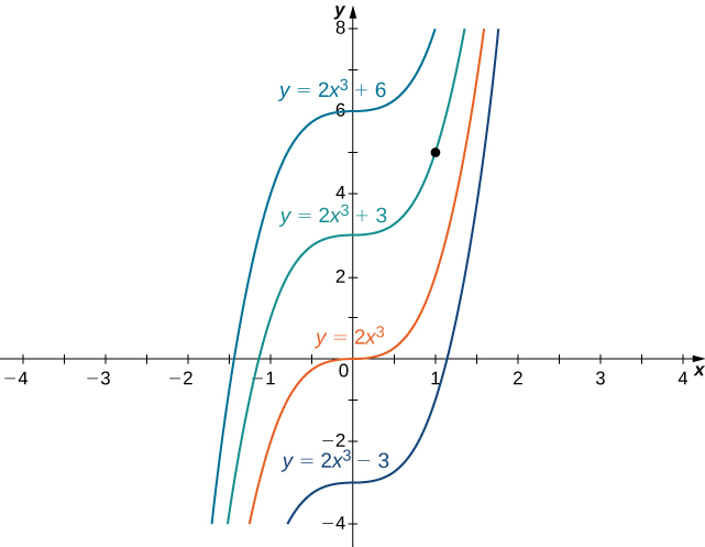
Figure \(\PageIndex{2}\): Some of the solution curves of the differential equation \(\dfrac{dy}{dx}=6x^2\) are displayed. The function \(y=2x^3+3\) satisfies the differential equation and the initial condition \(y(1)=5.\)

Example \(\PageIndex{2}\): Solving an Initial-Value Problem

Solve the initial-value problem

\[\dfrac{dy}{dx}=\sin (x),\quad \text{with } y(0)=5 \nonumber \]

Solution

First, we need to solve the differential equation. If \(\dfrac{dy}{dx}=\sin (x)\), then \(y=−\cos (x)+C\).

Next ,we need to look for a solution \(y\) that satisfies the initial condition. The initial condition \(y(0)=5\) means we need a constant \(C\) such that

\[y(0)=-\cos (0)+C=5 \implies -1+C= 5 \implies C=6 \nonumber \]

Thus, the solution of the initial-value problem is \(\boxed{y=-\cos (x)+6}\)

Exercise \(\PageIndex{2}\)

Solve the initial value problem \(\dfrac{dy}{dx}=3x^{-2}\) with \(y(1)=2\)

Answer

\(y=−\dfrac{3}{x}+5\)

Initial-value problems arise in many applications. Next we consider a problem in which a driver applies the brakes in a car. We are interested in how long it takes for the car to stop. Recall that the velocity function \(v(t)\) is the derivative of a position function \(s(t),\) and the acceleration \(a(t)\) is the derivative of the velocity function. In earlier examples in the text, we could calculate the velocity from the position and then compute the acceleration from the velocity. In the next example we work the other way around. Given an acceleration function, we calculate the velocity function. We then use the velocity function to determine the position function.

Example \(\PageIndex{3}\)

A car is traveling at the rate of \(60\) ft/sec when the brakes are applied. The car begins decelerating at a constant rate of \(10\) ft/sec².

1. How many seconds elapse before the car stops?
2. How far does the car travel during that time?

Solution

a. First we introduce variables for this problem. Let \(t\) be the time (in seconds) after the brakes are first applied. Let \(a(t)\) be the acceleration of the car (in feet per seconds squared) at time \(t\). Let \(v(t)\) be the velocity of the car (in feet per second) at time \(t\). Let \(s(t)\) be the car’s position (in feet) beyond the point where the brakes are applied at time \(t\).

The car is traveling at a rate of \(60\) ft/sec. Therefore, the initial velocity is \(v(0)=60\) ft/sec. Since the car is decelerating, the acceleration is \(a(t)=-10\) ft/s^2\). Since the acceleration is the derivative of the velocity, we have \(v′(t)=-10\).

Therefore, we have an initial-value problem to solve:

\(v′(t)=-10,\, v(0)=60\)

This constant has simple anti-derivative:

\(v(t)=-10t+C\)

Since \(v(0)=60\), we can see that \(v(0)=-10\cdot 0+C \implies C=60.\) Thus, the velocity function is

\(v(t)=−10t+60\)

To find how long it takes for the car to stop, we need to find the time t such that the velocity is zero.

Solving \(-10t+60=0,\) we obtain \(\boxed{t=6 \text{ seconds}}\).

b. To find how far the car travels during this time, we need to find the position of the car after \(6\) sec. We know the velocity \(v(t)\) is the derivative of the position \(s(t)\). Consider the initial position to be \(s(0)=0\). Therefore, we need to solve the initial-value problem

\(s′(t)=-10t+60,\, s(0)=0\)

We use \(D\) to represents the (possibliy different) constant when taking this anti-derivative:

\(s(t)=-10\cdot \dfrac{1}{2}t^2+60\cdot t+D =-5t^2+60t+D\)

Since \(s(0)=0\), we see that \(s(0)=-5\cdot 0^2+60\cdot 0+D \implies D=0\). Therefore, the position function is

\(s(t)=-5t^2+60t\)

Plugging in \(t=6\), we have \(s(6)=180\). Therefore, the car stops after a distance of \(\boxed{180 \text{ feet}}\).

Exercise \(\PageIndex{3}\)

Suppose the car is decelerating at the rate of \(6\) ft/sec\(^2\). How long does it take for the car to stop? How far will the car travel?

Answer

The car will stop in \(10\) seconds, traveling \(300\) feet.

Key Concepts

• If \(F\) is an anti-derivative of \(f\), then every anti-derivative of \(f\) is of the form \(F(x)+C\) for some constant \(C\).
• Solving the initial-value problem \[\dfrac{dy}{dx}=f(x),y(x_0)=y_0 \nonumber\]
• requires us first to find the set of anti-derivatives of \(f\) and then to look for the particular anti-derivative that also satisfies the initial condition.

Glossary

anti-derivative

a function \(F\) such that \(F′(x)=f(x)\) for all \(x\) in the domain of \(f\) is an anti-derivative of \(f\)

initial value problem

a problem that requires finding a function \(y\) that satisfies the differential equation \(\dfrac{dy}{dx}=f(x)\) together with the initial condition \(y(x_0)=y_0\)