
6.03: Linear Regression
- Page ID
- 126417

\( \newcommand{\vecs}[1]{\overset { \scriptstyle \rightharpoonup} {\mathbf{#1}} } \)
\( \newcommand{\vecd}[1]{\overset{-\!-\!\rightharpoonup}{\vphantom{a}\smash {#1}}} \)
\( \newcommand{\dsum}{\displaystyle\sum\limits} \)
\( \newcommand{\dint}{\displaystyle\int\limits} \)
\( \newcommand{\dlim}{\displaystyle\lim\limits} \)
\( \newcommand{\id}{\mathrm{id}}\) \( \newcommand{\Span}{\mathrm{span}}\)
( \newcommand{\kernel}{\mathrm{null}\,}\) \( \newcommand{\range}{\mathrm{range}\,}\)
\( \newcommand{\RealPart}{\mathrm{Re}}\) \( \newcommand{\ImaginaryPart}{\mathrm{Im}}\)
\( \newcommand{\Argument}{\mathrm{Arg}}\) \( \newcommand{\norm}[1]{\| #1 \|}\)
\( \newcommand{\inner}[2]{\langle #1, #2 \rangle}\)
\( \newcommand{\Span}{\mathrm{span}}\)
\( \newcommand{\id}{\mathrm{id}}\)
\( \newcommand{\Span}{\mathrm{span}}\)
\( \newcommand{\kernel}{\mathrm{null}\,}\)
\( \newcommand{\range}{\mathrm{range}\,}\)
\( \newcommand{\RealPart}{\mathrm{Re}}\)
\( \newcommand{\ImaginaryPart}{\mathrm{Im}}\)
\( \newcommand{\Argument}{\mathrm{Arg}}\)
\( \newcommand{\norm}[1]{\| #1 \|}\)
\( \newcommand{\inner}[2]{\langle #1, #2 \rangle}\)
\( \newcommand{\Span}{\mathrm{span}}\) \( \newcommand{\AA}{\unicode[.8,0]{x212B}}\)
\( \newcommand{\vectorA}[1]{\vec{#1}} % arrow\)
\( \newcommand{\vectorAt}[1]{\vec{\text{#1}}} % arrow\)
\( \newcommand{\vectorB}[1]{\overset { \scriptstyle \rightharpoonup} {\mathbf{#1}} } \)
\( \newcommand{\vectorC}[1]{\textbf{#1}} \)
\( \newcommand{\vectorD}[1]{\overrightarrow{#1}} \)
\( \newcommand{\vectorDt}[1]{\overrightarrow{\text{#1}}} \)
\( \newcommand{\vectE}[1]{\overset{-\!-\!\rightharpoonup}{\vphantom{a}\smash{\mathbf {#1}}}} \)
\( \newcommand{\vecs}[1]{\overset { \scriptstyle \rightharpoonup} {\mathbf{#1}} } \)
\(\newcommand{\longvect}{\overrightarrow}\)
\( \newcommand{\vecd}[1]{\overset{-\!-\!\rightharpoonup}{\vphantom{a}\smash {#1}}} \)
\(\newcommand{\avec}{\mathbf a}\) \(\newcommand{\bvec}{\mathbf b}\) \(\newcommand{\cvec}{\mathbf c}\) \(\newcommand{\dvec}{\mathbf d}\) \(\newcommand{\dtil}{\widetilde{\mathbf d}}\) \(\newcommand{\evec}{\mathbf e}\) \(\newcommand{\fvec}{\mathbf f}\) \(\newcommand{\nvec}{\mathbf n}\) \(\newcommand{\pvec}{\mathbf p}\) \(\newcommand{\qvec}{\mathbf q}\) \(\newcommand{\svec}{\mathbf s}\) \(\newcommand{\tvec}{\mathbf t}\) \(\newcommand{\uvec}{\mathbf u}\) \(\newcommand{\vvec}{\mathbf v}\) \(\newcommand{\wvec}{\mathbf w}\) \(\newcommand{\xvec}{\mathbf x}\) \(\newcommand{\yvec}{\mathbf y}\) \(\newcommand{\zvec}{\mathbf z}\) \(\newcommand{\rvec}{\mathbf r}\) \(\newcommand{\mvec}{\mathbf m}\) \(\newcommand{\zerovec}{\mathbf 0}\) \(\newcommand{\onevec}{\mathbf 1}\) \(\newcommand{\real}{\mathbb R}\) \(\newcommand{\twovec}[2]{\left[\begin{array}{r}#1 \\ #2 \end{array}\right]}\) \(\newcommand{\ctwovec}[2]{\left[\begin{array}{c}#1 \\ #2 \end{array}\right]}\) \(\newcommand{\threevec}[3]{\left[\begin{array}{r}#1 \\ #2 \\ #3 \end{array}\right]}\) \(\newcommand{\cthreevec}[3]{\left[\begin{array}{c}#1 \\ #2 \\ #3 \end{array}\right]}\) \(\newcommand{\fourvec}[4]{\left[\begin{array}{r}#1 \\ #2 \\ #3 \\ #4 \end{array}\right]}\) \(\newcommand{\cfourvec}[4]{\left[\begin{array}{c}#1 \\ #2 \\ #3 \\ #4 \end{array}\right]}\) \(\newcommand{\fivevec}[5]{\left[\begin{array}{r}#1 \\ #2 \\ #3 \\ #4 \\ #5 \\ \end{array}\right]}\) \(\newcommand{\cfivevec}[5]{\left[\begin{array}{c}#1 \\ #2 \\ #3 \\ #4 \\ #5 \\ \end{array}\right]}\) \(\newcommand{\mattwo}[4]{\left[\begin{array}{rr}#1 \amp #2 \\ #3 \amp #4 \\ \end{array}\right]}\) \(\newcommand{\laspan}[1]{\text{Span}\{#1\}}\) \(\newcommand{\bcal}{\cal B}\) \(\newcommand{\ccal}{\cal C}\) \(\newcommand{\scal}{\cal S}\) \(\newcommand{\wcal}{\cal W}\) \(\newcommand{\ecal}{\cal E}\) \(\newcommand{\coords}[2]{\left\{#1\right\}_{#2}}\) \(\newcommand{\gray}[1]{\color{gray}{#1}}\) \(\newcommand{\lgray}[1]{\color{lightgray}{#1}}\) \(\newcommand{\rank}{\operatorname{rank}}\) \(\newcommand{\row}{\text{Row}}\) \(\newcommand{\col}{\text{Col}}\) \(\renewcommand{\row}{\text{Row}}\) \(\newcommand{\nul}{\text{Nul}}\) \(\newcommand{\var}{\text{Var}}\) \(\newcommand{\corr}{\text{corr}}\) \(\newcommand{\len}[1]{\left|#1\right|}\) \(\newcommand{\bbar}{\overline{\bvec}}\) \(\newcommand{\bhat}{\widehat{\bvec}}\) \(\newcommand{\bperp}{\bvec^\perp}\) \(\newcommand{\xhat}{\widehat{\xvec}}\) \(\newcommand{\vhat}{\widehat{\vvec}}\) \(\newcommand{\uhat}{\widehat{\uvec}}\) \(\newcommand{\what}{\widehat{\wvec}}\) \(\newcommand{\Sighat}{\widehat{\Sigma}}\) \(\newcommand{\lt}{<}\) \(\newcommand{\gt}{>}\) \(\newcommand{\amp}{&}\) \(\definecolor{fillinmathshade}{gray}{0.9}\)Lesson 1: Introduction to Linear Regression
Learning Objectives
After successful completion of this lesson, you should be able to:
1) Define a residual for a linear regression model,
2) Explain the concept of the least-squares method as an optimization approach,
3) Explain why other criteria of finding the regression model do not work.
Introduction
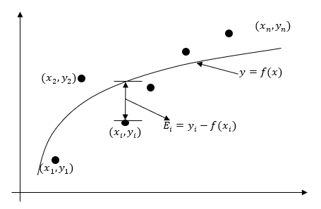
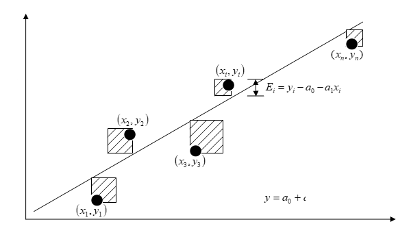
The problem statement for a regression model is as follows. Given \({n}\) data pairs \(\left( x_{1},y_{1} \right), \left( x_{2},y_{2} \right), \ldots, \left( x_{n},y_{n} \right)\), best fit \(y = f\left( x \right)\) to the data (Figure \(\PageIndex{1.1}\)).
Linear regression is the most popular regression model. In this model, we wish to predict response to \(n\) data points \(\left( x_{1},y_{1} \right),\left( x_{2},y_{2} \right),\ldots\ldots,\left( x_{n},y_{n} \right)\) by a regression model given by
\[y = a_{0} + a_{1}x\;\;\;\;\;\;\;\;\;\;\;\; (\PageIndex{1.1}) \nonumber\]
where \(a_{0}\) and \(a_{1}\) are the constants of the regression model.
A measure of goodness of fit, that is, how well \(a_{0} + a_{1}x\) predicts the response variable \(y\), is the magnitude of the residual \(E_{i}\) at each of the \(n\) data points.
\[E_{i} = y_{i} - \left( a_{0} + a_{1}x_{i} \right)\;\;\;\;\;\;\;\;\;\;\;\;(\PageIndex{1.2}) \nonumber\]
Ideally, if all the residuals \(E_{i}\) are zero, one has found an equation in which all the points lie on the model. Thus, minimization of the residuals is an objective of obtaining regression coefficients.
The most popular method to minimize the residual is the least-squares method, where the estimates of the constants of the models are chosen such that the sum of the squared residuals is minimized, that is, minimize
\[S_{r}=\sum_{i = 1}^{n}{E_{i}}^{2}\;\;\;\;\;\;\;\;\;\;\;\; (\PageIndex{1.3}) \nonumber\]
Why minimize the sum of the square of the residuals, \(S_{r}\)?
Why not, for instance, minimize the sum of the residual errors or the sum of the absolute values of the residuals? Alternatively, constants of the model can be chosen such that the average residual is zero without making individual residuals small. Would any of these criteria yield unbiased parameters with the smallest variance? All of these questions will be answered. Look at the example data in Table \(\PageIndex{1.1}\).
| \(x\) | \(y\) |
|---|---|
| \(2.0\) | \(4.0\) |
| \(3.0\) | \(6.0\) |
| \(2.0\) | \(6.0\) |
| \(3.0\) | \(8.0\) |
To explain this data by a straight line regression model,
\[y = a_{0} + a_{1}x\;\;\;\;\;\;\;\;\;\;\;\;(\PageIndex{1.4}) \nonumber\]
Let us use minimizing \(\displaystyle \sum_{i = 1}^{n}E_{i}\) as a criterion to find \(a_{0}\) and \(a_{1}\). Assume randomly that
\[y = 4x - 4\;\;\;\;\;\;\;\;\;\;\;\;(\PageIndex{1.5}) \nonumber\]
as the resulting regression model (Figure \(\PageIndex{1.2}\)).
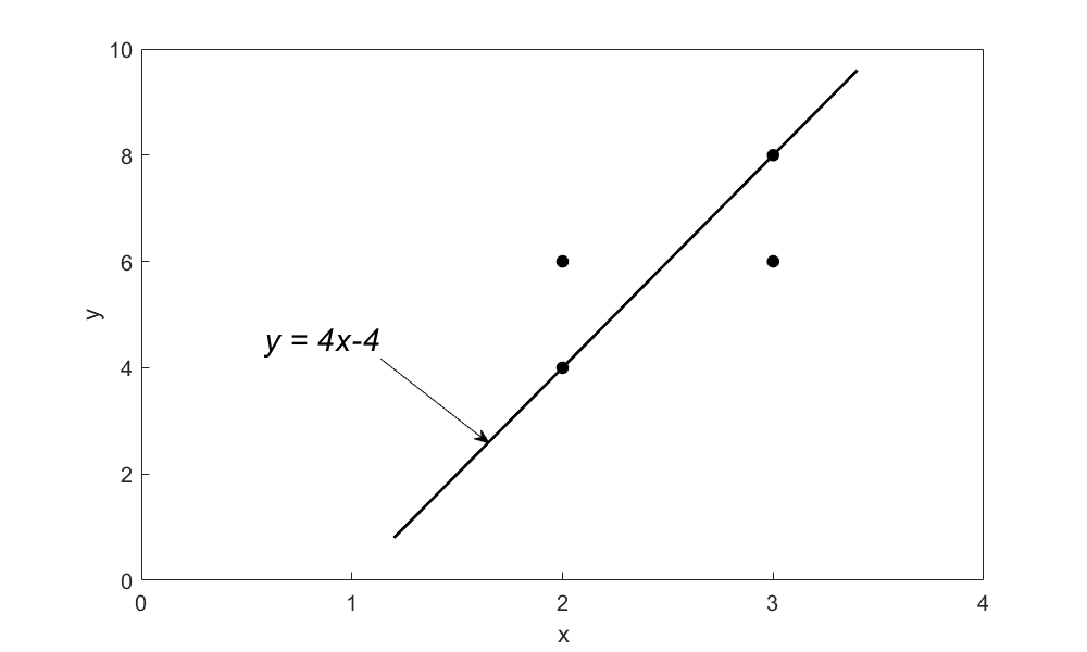
The sum of the residuals \(\displaystyle \sum_{i = 1}^{4}{E_{i}}^{} = 0\) is shown in Table \(\PageIndex{2.2}\).
| \(x\) | \(y\) | \(y_{predicted}\) | \(E = y - y_{predicted}\) |
|---|---|---|---|
| \(2.0\) | \(4.0\) | \(4.0\) | \(0.0\) |
| \(3.0\) | \(6.0\) | \(8.0\) | \(-2.0\) |
| \(2.0\) | \(6.0\) | \(4.0\) | \(2.0\) |
| \(3.0\) | \(8.0\) | \(8.0\) | \(0.0\) |
| \(\displaystyle \sum_{i = 1}^{4}E_{i} = 0\) |
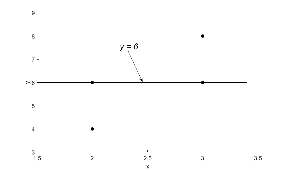
So does this give us the smallest possible sum of residuals? For this data, it does as \(\displaystyle \sum_{i = 1}^{4}E_{i} = 0,\) and it cannot be made any smaller. But does it give unique values for the parameters of the regression model? No, because, for example, a straight-line model (Figure \(\PageIndex{1.3}\))
\[y = 6\;\;\;\;\;\;\;\;\;\;\;\;(\PageIndex{1.6}) \nonumber\]
also gives \(\displaystyle \sum_{i = 1}^{4}E_{i} = 0\) as shown in Table \(\PageIndex{1.3}\).
In fact, there are many other straight lines for this data for which the sum of the residuals \(\displaystyle \sum_{i = 1}^{4}E_{i} = 0\). We hence find the regression models are not unique, and therefore this criterion of minimizing the sum of the residuals is a bad one.
| \(x\) | \(y\) | \(y_{\text{predicted}}\) | \(E = y - y_{predicted}\) |
|---|---|---|---|
| \(2.0\) | \(4.0\) | \(6.0\) | \(-2.0\) |
| \(3.0\) | \(6.0\) | \(6.0\) | \(0.0\) |
| \(2.0\) | \(6.0\) | \(6.0\) | \(0.0\) |
| \(3.0\) | \(8.0\) | \(6.0\) | \(2.0\) |
| \(\displaystyle \sum_{i = 1}^{4}E_{i} = 0\) |
You may think that the reason the criterion of minimizing \(\displaystyle \sum_{i = 1}^{n}E_{i}\) does not work is because negative residuals cancel with positive residuals. So, is minimizing the sum of absolute values of the residuals, that is, \(\displaystyle \sum_{i = 1}^{n}\left| E_{i} \right|\) better? Let us look at the same example data given in Table \(\PageIndex{1.1}\). For the regression model \(y = 4x - 4\), the sum of the absolute value of residuals \(\displaystyle \sum_{i = 1}^{4}\left| E_{i} \right| = 4\) is shown in Table \(\PageIndex{1.4}\).
| \(x\) | \(y\) | \(y_{predicted}\) | \(E = y - y_{predicted}\) |
|---|---|---|---|
| \(2.0\) | \(4.0\) | \(4.0\) | \(0.0\) |
| \(3.0\) | \(6.0\) | \(8.0\) | \(2.0\) |
| \(2.0\) | \(6.0\) | \(4.0\) | \(2.0\) |
| \(3.0\) | \(8.0\) | \(8.0\) | \(0.0\) |
| \(\displaystyle \sum_{i = 1}^{4}\left| E_{i} \right| = 4\) |
The value of \(\displaystyle \sum_{i = 1}^{4}\left| E_{i} \right| = 4\) also exists for the straight-line model \(y = 6.\) (see Table \(\PageIndex{1.5}\)).
| \(x\) | \(y\) | \(y_{predicted}\) | \(E = y - y_{predicted}\) |
|---|---|---|---|
| \(2.0\) | \(4.0\) | \(6.0\) | \(-2.0\) |
| \(3.0\) | \(6.0\) | \(6.0\) | \(0.0\) |
| \(2.0\) | \(6.0\) | \(6.0\) | \(0.0\) |
| \(3.0\) | \(8.0\) | \(6.0\) | \(2.0\) |
| \(\displaystyle \sum_{i = 1}^{4}{|E_{i}}| = 4\) |
No other straight-line model that you may choose for this data has\(\displaystyle \sum_{i = 1}^{4}\left| E_{i} \right| < 4\). And there are many other straight lines for which the sum of absolute values of the residuals \(\displaystyle \sum_{i = 1}^{4}\left| E_{i} \right| = 4\). We hence find that the regression models are not unique, and hence the criterion of minimizing the sum of the absolute values of the residuals is also a bad one.
To get a unique regression model, the least-squares criterion where we minimize the sum of the square of the residuals
\[\begin{split} S_{r} &= \sum_{i = 1}^{n}{E_{i}}^{2}\\ &= \sum_{i = 1}^{n}(y_i-a_0- a_1x_i)^{2}\;\;\;\;\;\;\;\;\;\;\;\;(\PageIndex{1.7}) \end{split}\]
is recommended. The formulas obtained for the regression constants \(a_0\) and \(a_1\) are given below and will be derived in the next lesson.
\[\displaystyle a_{0} = \frac{\displaystyle\sum_{i = 1}^{n}y_{i}\sum_{i = 1}^{n}x_{i}^{2} - \sum_{i = 1}^{n}x_{i}\sum_{i = 1}^{n}{x_{i}y_{i}}}{\displaystyle n\sum_{i = 1}^{n}x_{i}^{2} \ -\left( \sum_{i = 1}^{n}x_{i} \right)^{2}}\;\;\;\;\;\;\;\;\;\;\;\; (\PageIndex{1.8}) \nonumber\]
\[\displaystyle a_{1} = \frac{\displaystyle n\sum_{i = 1}^{n}{x_{i}y_{i}} - \sum_{i = 1}^{n}x_{i}\sum_{i = 1}^{n}y_{i}}{\displaystyle n\sum_{i = 1}^{n}x_{i}^{2}-\left( \sum_{i = 1}^{n}x_{i} \right)^{2}}\;\;\;\;\;\;\;\;\;\;\;\; (\PageIndex{1.9}) \nonumber\]
The formula for \(a_0\) can also be written as
\[\begin {split} \displaystyle a_{0} &= \frac{\displaystyle \sum_{i = 1}^{n}y_{i}}{n} -a_1\frac{\displaystyle \sum_{i = 1}^{n}x_{i}}{n} \\ &= \bar{y} - a_{1}\bar{x} \end{split}\;\;\;\;\;\;\;\;\;\;\;\; (\PageIndex{1.10}) \nonumber\]
Audiovisual Lecture
Title: Linear Regression - Background
Summary: This video is about learning the background of linear regression of how the minimization criterion is selected to find the constants of the model.
Lesson 2: Straight-Line Regression Model without an Intercept
Learning Objectives
After successful completion of this lesson, you should be able to:
1) derive constants of linear regression model without an intercept,
2) use the derived formula to find the constants of the nonlinear regression model from given data.
Introduction
In this model, we wish to predict response to \(n\) data points \(\left( x_{1},y_{1} \right),\left( x_{2},y_{2} \right),\ldots\ldots,\left( x_{n},y_{n} \right)\) by a regression model given by
\[y = a_{1}x\;\;\;\;\;\;\;\;\;\;\;\;(\PageIndex{2.1}) \nonumber\]
where \(a_{1}\) is the only constant of the regression model.
A measure of goodness of fit, that is, how well \(a_{1}x\) predicts the response variable \(y\) is the sum of the square of the residuals, \(S_{r}\)
\[\begin{split} S_{r} &= \sum_{i = 1}^{n}{E_{i}}^{2}\\ &= \sum_{i = 1}^{n}\left( y_{i} - a_{1}x_{i} \right)^{2}\;\;\;\;\;\;\;\;\;\;\;\; (\PageIndex{2.2}) \end{split}\]
To find \(a_{1},\) we look for the value of \(a_{1}\) for which \(S_{r}\) is the absolute minimum.
We will begin by conducting the first derivative test. Take the derivative of Equation \((\PageIndex{2.2})\)
\[\frac{dS_{r}}{da_{1}} = 2\sum_{i = 1}^{n}{\left( y_{i} - a_{1}x_{i} \right)\left( - x_{i} \right)} = 0\;\;\;\;\;\;\;\;\;\;\;\; (\PageIndex{2.3}) \nonumber\]
Now putting
\[\frac{dS_{r}}{da_{1}} = 0 \nonumber\]
gives
\[2\sum_{i = 1}^{n}{\left( y_{i} - a_{1}x_{i} \right)\left( - x_{i} \right)} = 0 \nonumber\]
giving
\[- 2\sum_{i = 1}^{n}{y_{i}x_{i} + 2\sum_{i = 1}^{n}{a_{1}x_{i}^{2}}} = 0 \nonumber\]
\[- 2\sum_{i = 1}^{n}{y_{i}x_{i} + {2a}_{1}\sum_{i = 1}^{n}x_{i}^{2}} = 0 \nonumber\]
Solving the above equation for \(a_{1}\) gives
\[a_{1} = \frac{\displaystyle \sum_{i = 1}^{n}{y_{i}x_{i}}}{\displaystyle \sum_{i = 1}^{n}x_{i}^{2}}\;\;\;\;\;\;\;\;\;\;\;\;(\PageIndex{2.4}) \nonumber\]
Let’s conduct the second derivative test.
\[\begin{split} \frac{d^{2}S_{r}}{d{a_{1}}^{2}} &= \frac{d}{da_{1}}\left( 2\sum_{i = 1}^{n}{\left( y_{i} - a_{1}x_{i} \right)\left( - x_{i} \right)} \right)\\ &= \frac{d}{da_{1}} \sum_{i = 1}^{n} (-2 x_{i}y_{i} + 2a_{1}{x_{i}}^{2}) \\ &= \sum_{i = 1}^{n} 2x_{i}^{2} > 0\;\;\;\;\;\;\;\;\;\;\;\; (\PageIndex{2.5}) \end{split}\]
for at most one \(x_{i} \neq 0,\) which is a pragmatic assumption that all the \(x\)-values are not zero.
This inequality shows that the Equation \((\PageIndex{2.2})\) value of \(a_{1}\) corresponds to a location of local minimum. Since the sum of the squares of the residuals, \(S_{r}\) is a continuous function of \(a_{1}\), that \(S_r\) has only one point where \(\displaystyle \frac{dS_{r}}{da_{1}} = 0,\) and at that point, we have \(\displaystyle \frac{d^{2}S_{r}}{d{a_{1}}^{2}} > 0\), it corresponds not only to a local minimum but an absolute minimum as well. Hence, Equation \((\PageIndex{2.4})\) gives us the value of the constant, \(a_1\), of the regression model \(y=a_1x\).
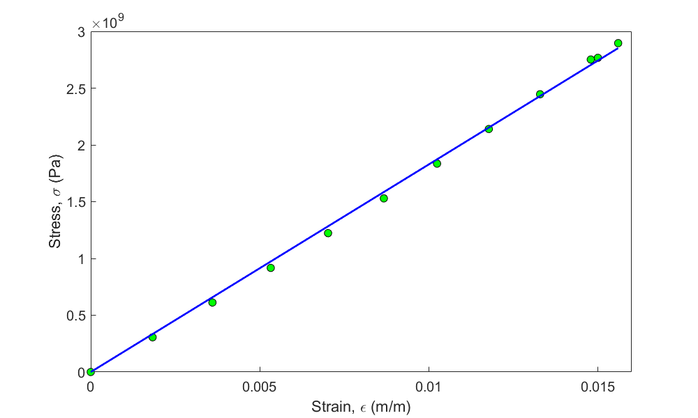
To find the longitudinal modulus of a composite material, the following data, as given in Table \(\PageIndex{2.1}\), is collected.
|
Strain (%) |
Stress (\(\text{MPa}\)) |
|---|---|
| \(0\) | \(0\) |
| \(0.183\) | \(306\) |
| \(0.36\) | \(612\) |
| \(0.5324\) | \(917\) |
| \(0.702\) | \(1223\) |
| \(0.867\) | \(1529\) |
| \(1.0244\) | \(1835\) |
| \(1.1774\) | \(2140\) |
| \(1.329\) | \(2446\) |
| \(1.479\) | \(2752\) |
| \(1.5\) | \(2767\) |
| \(1.56\) | \(2896\) |
Find the longitudinal modulus \(E\) using the following regression model:
\[\sigma = E\varepsilon \nonumber\]
Solution
Rewriting data from Table \(\PageIndex{2.1}\) in the base SI system of units is given in Table \(\PageIndex{2.2}\).
|
Strain (\(\text{m/m}\)) |
Stress (\(\text{Pa}\)) |
|---|---|
| \(0.0000\) | \(0.0000\) |
| \(1.8300 \times 10^{- 3}\) | \(3.0600 \times 10^{8}\) |
| \(3.6000 \times 10^{- 3}\) | \(6.1200 \times 10^{8}\) |
| \(5.3240 \times 10^{- 3}\) | \(9.1700 \times 10^{8}\) |
| \(7.0200 \times 10^{- 3}\) | \(1.2230 \times 10^{9}\) |
| \(8.6700 \times 10^{- 3}\) | \(1.5290 \times 10^{9}\) |
| \(1.0244 \times 10^{- 2}\) | \(1.8350 \times 10^{9}\) |
| \(1.1774 \times 10^{- 2}\) | \(2.1400 \times 10^{9}\) |
| \(1.3290 \times 10^{- 2}\) | \(2.4460 \times 10^{9}\) |
| \(1.4790 \times 10^{- 2}\) | \(2.7520 \times 10^{9}\) |
| \(1.5000 \times 10^{- 2}\) | \(2.7670 \times 10^{9}\) |
| \(1.5600 \times 10^{- 2}\) | \(2.8960 \times 10^{9}\) |
Using Equation \((\PageIndex{2.4})\) gives
\[E = \frac{\displaystyle \sum_{i = 1}^{n}{\sigma_{i}\varepsilon_{i}}}{\displaystyle \sum_{i = 1}^{n}{\varepsilon_{i}}^{2}}\;\;\;\;\;\;\;\;\;\;\;\;(\PageIndex{2.E1.1}) \nonumber\]
The summations used in Equation \((\PageIndex{2.E1.1})\) are given in Table \(\PageIndex{2.3}\).
| \(i\) | \(\varepsilon\) | \(\sigma\) | \(\varepsilon^2\) | \(\varepsilon\sigma\) |
|---|---|---|---|---|
| \(1\) | \(0.0000\) | \(0.0000\) | \(0.0000\) | \(0.0000\) |
| \(2\) | \(1.8300\times10^{-3}\) | \(3.0600\times10^8\) | \(3.3489\times10^{-6}\) | \(5.5998\times10^5\) |
| \(3\) | \(3.6000\times10^{-3}\) | \(6.1200\times10^8\) | \(1.2960\times10^{-5}\) | \(2.2032\times10^6\) |
| \(4\) | \(5.3240\times10^{-3}\) | \(9.1700\times10^8\) | \(2.8345\times10^{-5}\) | \(4.8821\times10^6\) |
| \(5\) | \(7.0200\times10^{-3}\) | \(1.2230\times10^9\) | \(4.9280\times10^{-5}\) | \(8.5855\times10^6\) |
| \(6\) | \(8.6700\times10^{-3}\) | \(1.5290\times10^9\) | \(7.5169\times10^{-5}\) | \(1.3256\times10^7\) |
| \(7\) | \(1.0244\times10^{-2}\) | \(1.8350\times10^9\) | \(1.0494\times10^{-4}\) | \(1.8798\times10^7\) |
| \(8\) | \(1.1774\times10^{-2}\) | \(2.1400\times10^9\) | \(1.3863\times10^{-4}\) | \(2.5196\times10^7\) |
| \(9\) | \(1.3290\times10^{-2}\) | \(2.4460\times10^9\) | \(1.7662\times10^{-4}\) | \(3.2507\times10^7\) |
| \(10\) | \(1.4790\times10^{-2}\) | \(2.7520\times10^9\) | \(2.1874\times10^{-4}\) | \(4.0702\times10^7\) |
| \(11\) | \(1.5000\times10^{-2}\) | \(2.7670\times10^9\) | \(2.2500\times10^{-4}\) | \(4.1505\times10^7\) |
| \(12\) | \(1.5600\times10^{-2}\) | \(2.8960\times10^9\) | \(2.4336\times10^{-4}\) | \(4.5178\times10^7\) |
| \(\displaystyle \sum_{i=1}^{12}\) | \(1.2764\times10^{-3}\) | \(2.3337\times10^8\) |
\[n = 12 \nonumber\]
\[\sum_{i = 1}^{12}{\varepsilon_{i}^{2} = 1.2764 \times 10^{- 3}} \nonumber\]
\[\sum_{i = 1}^{12}{\sigma_{i}\varepsilon_{i} = 2.3337 \times 10^{8}} \nonumber\]
From Equation \((\PageIndex{2.E1.1})\)
\[\begin{split} E &= \frac{\displaystyle \sum_{i = 1}^{12}{\sigma_{i}\varepsilon_{i}}}{\displaystyle \sum_{i = 1}^{12}{\varepsilon_{i}}^{2}} \\ &= \frac{2.3337 \times 10^{8}}{1.2764 \times 10^{- 3}}\\ &= 1.8284 \times 10^{11}\ \text{Pa}\\ &= 182.84 \text{ GPa}\end{split}\]
Audiovisual Lecture
Title: Linear Regression with Zero Intercept: Derivation
Summary: This video discusses how to regress data to a linear polynomial with zero constant term (no intercept). This segment shows you the derivation and also explains why using the formula for a general straight line is not valid for this case.
Audiovisual Lecture
Title: Linear Regression with Zero Intercept: Example
Summary: This video shows an example of how to conduct linear regression with zero intercept.
Lesson 3: Theory of General Straight-Line Regression Model
Learning Objectives
After successful completion of this lesson, you should be able to:
1) derive the constants of a linear regression model based on the least-squares method criterion.
Introduction
In this model, we best fit a general straight line \(y=a_0 +a_1x\) to the \(n\) data points \((x_1,y_1),\ (x_2,y_2),\ldots,\ (x_n,y_n)\)
Let us use the least-squares criterion where we minimize the sum of the square of the residuals, \(S_{r}\):
\[\begin{split} S_{r} &= \sum_{i = 1}^{n}{E_{i}}^{2}\\&= \sum_{i = 1}^{n}\left( y_{i} - a_{0} - a_{1}x_{i} \right)^{2}\;\;\;\;\;\;\;\;\;\;\;\; (\PageIndex{3.1}) \end{split}\]
To find \(a_{0}\) and \(a_{1}\), we need to calculate where the sum of the square of the residuals, \(S_{r}\) is the absolute minimum. We start this process of finding the absolute minimum first by
- taking the partial derivative of \(S_{r}\) with respect to \(a_{0}\) and \(a_{1}\) and set them equal to zero, and
- conducting the second derivative test.
Taking the partial derivative of \(S_{r}\) with respect to \(a_{0}\) and \(a_{1}\) and seting them equal to zero gives
\[\frac{\partial S_{r}}{\partial a_{0}} = 2\sum_{i = 1}^{n}{\left( y_{i} - a_{0} - a_{1}x_{i} \right)\left( - 1 \right)} = 0\;\;\;\;\;\;\;\;\;\;\;\; (\PageIndex{3.2}) \nonumber\]
\[\frac{\partial S_{r}}{\partial a_{1}} = 2\sum_{i = 1}^{n}{\left( y_{i} - a_{0} - a_{1}x_{i} \right)\left( - x_{i} \right)} = 0\;\;\;\;\;\;\;\;\;\;\;\; (\PageIndex{3.3}) \nonumber\]
Dividing both sides by \(2\) and expanding the summations in Equations \((\PageIndex{3.2})\) and \((\PageIndex{3.3})\) gives,
\[- \sum_{i = 1}^{n}{y_{i} + \sum_{i = 1}^{n}a_{0} + \sum_{i = 1}^{n}{a_{1}x_{i}}} = 0 \nonumber\]
\[- \sum_{i = 1}^{n}{y_{i}x_{i} + \sum_{i = 1}^{n}{a_{0}x_{i}} + \sum_{i = 1}^{n}{a_{1}x_{i}^{2}}} = 0 \nonumber\]
Noting that
\[\sum_{i = 1}^{n}a_{0} = a_{0} + a_{0} + \ldots + a_{0} = na_{0} \nonumber\]
we get
\[na_{0} + a_{1}\sum_{i = 1}^{n}x_{i} = \sum_{i = 1}^{n}y_{i}\;\;\;\;\;\;\;\;\;\;\;\; (\PageIndex{3.4}) \nonumber\]
\[a_{0}\sum_{i = 1}^{n}x_{i} + a_{1}\sum_{i = 1}^{n}x_{i}^{2} = \sum_{i = 1}^{n}{x_{i}y_{i}}\;\;\;\;\;\;\;\;\;\;\;\; (\PageIndex{3.5}) \nonumber\]
Solving the above two simultaneous linear equations \((\PageIndex{3.4})\) and \((\PageIndex{3.5})\) gives
\[a_{1} = \frac{n \displaystyle \sum_{i = 1}^{n}{x_{i}y_{i}} - \sum_{i = 1}^{n}x_{i} \sum_{i = 1}^{n}y_{i}}{n \displaystyle \sum_{i = 1}^{n}x_{i}^{2} - \left( \sum_{i = 1}^{n}x_{i} \right)^{2}}\;\;\;\;\;\;\;\;\;\;\;\; (\PageIndex{3.6}) \nonumber\]
\[a_{0} = \frac{\displaystyle \sum_{i = 1}^{n}x_{i}^{2}\ \sum_{i = 1}^{n}y_{i} - \sum_{i = 1}^{n}x_{i} \sum_{i = 1}^{n}{x_{i}y_{i}}}{n\displaystyle \sum_{i = 1}^{n}x_{i}^{2} - \left( \sum_{i = 1}^{n}x_{i} \right)^{2}}\;\;\;\;\;\;\;\;\;\;\;\; (\PageIndex{3.7}) \nonumber\]
Redefining
\[S_{xy} = \sum_{i = 1}^{n}{x_{i}y_{i}} - n\bar{x}\bar{y} \nonumber\]
\[S_{xx} = \sum_{i = 1}^{n}x_{i}^{2} - n \bar{x}^{2} \nonumber\]
\[\bar{x} = \frac{\displaystyle \sum_{i = 1}^{n}x_{i}}{n} \nonumber\]
\[\bar{y} = \frac{\displaystyle \sum_{i = 1}^{n}y_{i}}{n} \nonumber\]
we can also rewrite the constants \(a_{0}\) and \(a_{1}\) from Equations \((\PageIndex{3.6})\) and \((\PageIndex{3.7})\) as
\[a_{1} = \frac{S_{xy}}{S_{xx}}\;\;\;\;\;\;\;\;\;\;\;\; (\PageIndex{3.8}) \nonumber\]
\[a_{0} = \bar{y} - a_{1}\bar{x}\;\;\;\;\;\;\;\;\;\;\;\; (\PageIndex{3.9}) \nonumber\]
Putting the first derivative equations equal to zero only gives us a critical point. For a general function, it could be a local minimum, a local maximum, a saddle point, or none of the previous. The second derivative test, though, given in the “optional” appendix below, shows that it is a local minimum. Now, is this local minimum also the absolute minimum? Yes, because the first derivative test gave us only one solution, and that \(S_{r}\) is a continuous function of \(a_{0}\) and \(a_{1}\).
Appendix
Question
Given \(n\) data pairs, \(\left( x_{1},y_{1} \right),\ldots,\left( x_{n},y_{n} \right)\), do the values of the two constants \(a_{0\ }\)and \(a_{1}\)in the least-squares straight-line regression model \(y = a_{0} + a_{1}x\) correspond to the absolute minimum of the sum of the squares of the residuals? Are these constants of regression unique?
Solution
Given \(n\) data pairs\(\left( x_{1},y_{1} \right),\ldots,\left( x_{n},y_{n} \right)\), the best fit for the straight-line regression model
\[y = a_{0} + a_{1}x\;\;\;\;\;\;\;\;\;\;\;\; (\PageIndex{A.1}) \nonumber\]
is found by the method of least squares. Starting with the sum of the squares of the residuals \(S_{r}\)
\[S_{r} = \sum_{i = 1}^{n}\left( y_{i} - a_{0} - a_{1}x_{i} \right)^{2}\;\;\;\;\;\;\;\;\;\;\;\; (\PageIndex{A.2}) \nonumber\]
and using
\[\frac{\partial S_{r}}{\partial a_{0}} = 0\;\;\;\;\;\;\;\;\;\;\;\; (\PageIndex{A.3}) \nonumber\]
\[\frac{\partial S_{r}}{\partial a_{1}} = 0\;\;\;\;\;\;\;\;\;\;\;\; (\PageIndex{A.4}) \nonumber\]
gives two simultaneous linear equations whose solution is
\[a_{1} = \frac{\displaystyle n\sum_{i = 1}^{n}{x_{i}y_{i}} - \sum_{i = 1}^{n}x_{i}\sum_{i = 1}^{n}y_{i}}{\displaystyle n\sum_{i = 1}^{n}x_{i}^{2} - \left( \sum_{i = 1}^{n}x_{i} \right)^{2}}\;\;\;\;\;\;\;\;\;\;\;\; (\PageIndex{A.5a}) \nonumber\]
\[a_{0} = \frac{\displaystyle \sum_{i = 1}^{n}x_{i}^{2}\sum_{i = 1}^{n}y_{i} - \sum_{i = 1}^{n}x_{i}\sum_{i = 1}^{n}{x_{i}y_{i}}}{\displaystyle n\sum_{i = 1}^{n}x_{i}^{2} - \left( \sum_{i = 1}^{n}x_{i} \right)^{2}}\;\;\;\;\;\;\;\;\;\;\;\; (\PageIndex{A.5b}) \nonumber\]
But do these values of \(a_{0}\) and \(a_{1}\) give the absolute minimum value of \(S_{r}\) (Equation \((\PageIndex{A.2})\))? The first derivative analysis only tells us that these values give local minima or maxima of \(S_{r}\), and not whether they give an absolute minimum or maximum. So, we still need to figure out if they correspond to an absolute minimum.
We need first to conduct a second derivative test to find out whether the point \((a_{0},a_{1})\) from Equation \((\PageIndex{A.5})\) gives a local minimum of \(S_r\). Only then can we show if this local minimum also corresponds to the absolute minimum (or maximum).
What is the second derivative test for a local minimum of a function of two variables?
If you have a function \(f\left( x,y \right)\) and we found a critical point \(\left( a,b \right)\) from the first derivative test, then \(\left( a,b \right)\) is a minimum point if
\[\frac{\partial^{2}f}{\partial x^{2}}\frac{\partial^{2}f}{\partial y^{2}} - \left( \frac{\partial^{2}f}{\partial x\partial y} \right)^{2} > 0,\ \text{and}\;\;\;\;\;\;\;\;\;\;\;\; (\PageIndex{A.6}) \nonumber\]
\[\frac{\partial^{2}f}{\partial x^{2}} > 0\ \text{or}\ \frac{\partial^{2}f}{\partial y^{2}} > 0\;\;\;\;\;\;\;\;\;\;\;\; (\PageIndex{A.7}) \nonumber\]
From Equation \((\PageIndex{A.2})\)
\[\begin{split} \frac{\partial S_{r}}{\partial a_{0}} &= \sum_{i = 1}^{n}{2\left( y_{i} - a_{0} - a_{1}x_{i} \right)( - 1)}\\ &= - 2\sum_{i = 1}^{n}\left( y_{i} - a_{0} - a_{1}x_{i} \right)\;\;\;\;\;\;\;\;\;\;\;\; (\PageIndex{A.8}) \end{split}\]
\[\begin{split} \frac{\partial S_{r}}{\partial a_{1}} &= \sum_{i = 1}^{n}{2\left( y_{i} - a_{0} - a_{1}x_{i} \right)}( - x_{i})\\ &= - 2\sum_{i = 1}^{n}\left( x_{i}y_{i} - a_{0}x_{i} - a_{1}x_{i}^{2} \right)\;\;\;\;\;\;\;\;\;\;\;\; (\PageIndex{A.9}) \end{split}\]
then
\[\begin{split} \frac{\partial^{2}S_{r}}{\partial a_{0}^{2}} &= - 2\sum_{i = 1}^{n}{- 1}\\ &= 2n\;\;\;\;\;\;\;\;\;\;\;\; (\PageIndex{A.10}) \end{split}\]
\[\frac{\partial^{2}S_{r}}{\partial a_{1}^{2}} = 2\sum_{i = 1}^{n}x_{i}^{2}\;\;\;\;\;\;\;\;\;\;\;\; (\PageIndex{A.11}) \nonumber\]
\[\frac{\partial^{2}S_{r}}{\partial a_{0}\partial a_{1}} = 2\sum_{i = 1}^{n}x_{i}\;\;\;\;\;\;\;\;\;\;\;\; (\PageIndex{A.12}) \nonumber\]
So, we satisfy condition \((\PageIndex{A.7})\), because from Equation \((\PageIndex{A.10})\), we see that \(2n\) is a positive number. Although not required, from Equation \((\PageIndex{A.11})\), we see that \(\displaystyle 2\sum_{i = 1}^{n}{x_{i}^{2}\ }\)is also a positive number as assuming that all \(x\) data points are NOT zero is reasonable.
Is the other condition (Equation \((\PageIndex{A.6})\)) for \(S_{r}\) being a minimum met? Yes, we can show (proof not given that the term is positive)
\[\begin{split} \frac{\partial^{2}S_{r}}{\partial a_{0}^{2}}\frac{\partial^{2}S_{r}}{\partial a_{1}^{2}} - \left( \frac{\partial^{2}S_{r}}{\partial a_{0}\partial a_{1}} \right)^{2} &= \left( 2n \right)\left( 2\sum_{i = 1}^{n}x_{i}^{2} \right) - \left( 2\sum_{i = 1}^{n}x_{i} \right)^{2}\\ &= 4\left\lbrack n\sum_{i = 1}^{n}x_{i}^{2} - \left( \sum_{i = 1}^{n}x_{i} \right)^{2} \right\rbrack\\ &= 4\sum_{\begin{matrix} i = 1 \\ i < j \\ \end{matrix}}^{n}{(x_{i} - x_{j})^{2}} > 0\;\;\;\;\;\;\;\;\;\;\;\;\;\; (\PageIndex{A.13}) \end{split}\]
So, the values of \(a_{0}\) and \(a_{1}\) that we have in Equation \((\PageIndex{A.5})\) do correspond to a local minimum of \(S_r\). Now, is this local minimum also the absolute minimum? Yes, because the first derivative test gave us only one solution, and that \(S_{r}\) is a continuous function of \(a_{0}\) and \(a_{1}\).
As a side note, the denominator in Equations \((\PageIndex{A.5a})\) and \((\PageIndex{A.5b})\) is nonzero, as shown by Equation \((\PageIndex{A.13})\). This nonzero value proves that \(a_{0}\) and \(a_{1}\) are finite numbers.
Audiovisual Lecture
Title: Derivation of Linear Regression
Summary: This video is on learning how the linear regression formula is derived.
Lesson 4: Application of General Straight-Line Regression Model
Learning Objectives
After successful completion of this lesson, you should be able to:
1) calculate the constants of a linear regression model.
Recap
In the previous lesson, we derived the formulas for the linear regression model. In this lesson, we show the application of the formulas to an applied engineering problem.
The torque \(T\) needed to turn the torsional spring of a mousetrap through an angle, \(\theta\) is given below
|
\(Angle,\) \(\theta\) \(\text{Radians}\) |
\(Torque\), \(T\) \(\text{N} \cdot \text{m}\) |
|---|---|
| \(0.698132\) | \(0.188224\) |
| \(0.959931\) | \(0.209138\) |
| \(1.134464\) | \(0.230052\) |
| \(1.570796\) | \(0.250965\) |
| \(1.919862\) | \(0.313707\) |
Find the constants \(k_{1}\) and \(k_{2}\) of the regression model
\[T = k_{1} + k_{2}\theta\;\;\;\;\;\;\;\;\;\;\;\; (\PageIndex{4.E1.1}) \nonumber\]
Solution
For the linear regression model,
\[T = k_{1} + k_{2}\theta \nonumber\]
the constants of the regression model are given by
\[k_{2} = \frac{\displaystyle n\sum_{i = 1}^{5}{\theta_{i}T_{i}} - \sum_{i = 1}^{5}\theta_{i}\sum_{i = 1}^{5}T_{i}}{\displaystyle n\sum_{i = 1}^{5}\theta_{i}^{2} - \left( \sum_{i = 1}^{5}\theta_{i} \right)^{2}}\;\;\;\;\;\;\;\;\;\;\;\; (\PageIndex{4.E1.2}) \nonumber\]
\[k_{1} = \bar{T} - k_{2}\bar{\theta}\;\;\;\;\;\;\;\;\;\;\;\; (\PageIndex{4.E1.3}) \nonumber\]
Table \(\PageIndex{4.2}\) shows the summations needed for the calculation of the above two constants \(k_{1}\) and \(k_{2}\) of the regression model.
| \(i\) | \(\theta\) | \(T\) | \(\theta^2\) | \(T \theta\) |
|---|---|---|---|---|
| \(Radians\) | \(N \cdot m\) | \(Radians^2\) | \(N \cdot m\) | |
| \(1\) | \(0.698132\) | \(0.188224\) | \(4.87388 \times 10^{-1}\) | \(1.31405\times10^{-1}\) |
| \(2\) | \(0.959931\) | \(0.209138\) | \(9.21468 \times 10^{-1}\) | \(2.00758\times10^{-1}\) |
| \(3\) | \(1.134464\) | \(0.230052\) | \(1.2870\) | \(2.60986\times10^{-1}\) |
| \(4\) | \(1.570796\) | \(0.250965\) | \(2.4674\) | \(3.94215\times10^{-1}\) |
| \(5\) | \(1.919862\) | \(0.313707\) | \(3.6859\) | \(6.02274\times10^{-1}\) |
| \(\displaystyle \sum_{i = 1}^{5}\) | \(6.2831\) | \(1.1921\) | \(8.8491\) | \(1.5896\) |
Using the summations from the last row of Table \(\PageIndex{4.2}\), we get
\[n = 5 \nonumber\]
From Equation \((\PageIndex{4.E1.2})\),
\[\begin{split} k_{2} &= \frac{\displaystyle n\sum_{i = 1}^{5}{\theta_{i}T_{i}} - \sum_{i = 1}^{5}\theta_{i}\sum_{i = 1}^{5}T_{i}}{\displaystyle n\sum_{i = 1}^{5}\theta_{i}^{2} - \left( \sum_{i = 1}^{5}\theta_{i} \right)^{2}}\\[4pt] &= \frac{5(1.5896) - (6.2831)(1.1921)}{5(8.8491) - (6.2831)^{2}}\\[4pt] &= 9.6091 \times 10^{- 2}\text{N-m/rad} \end{split}\]
To find \(k_{1}\)
\[\begin{split} \bar{T} &= \frac{\displaystyle \sum_{i = 1}^{5}T_{i}}{n}\\ &= \frac{1.1921}{5}\\ &= 2.3842 \times 10^{- 1} N-m \end{split}\]
\[\begin{split} \bar{\theta} &= \frac{\displaystyle \sum_{i = 1}^{5}\theta_{i}}{n}\\ &= \frac{6.2831}{5}\\ &= 1.2566\ {radians} \end{split}\]
From Equation \((\PageIndex{4.E1.3})\),
\[\begin{split} k_{1} &= \bar{T} - k_{2}\bar{\theta}\\ &= 2.3842 \times 10^{- 1} - (9.6091 \times 10^{- 2})(1.2566)\\ &= 1.1767 \times 10^{- 1} \text{N-m} \end{split}\]
Audiovisual Lecture
Title: Linear Regression Applications
Summary: This video will teach you, through an example, how to regress data to a straight line.
Multiple Choice Test
(1). Given \(\left( x_{1},y_{1} \right),\left( x_{2},y_{2} \right),............,\left( x_{n},y_{n} \right),\) best fitting data to \(y = f\left( x \right)\) by least squares requires minimization of
(A) \(\displaystyle \sum_{i = 1}^{n}\left\lbrack y_{i} - f\left( x_{i} \right) \right\rbrack\)
(B) \(\displaystyle \sum_{i = 1}^{n}\left| y_{i} - f\left( x_{i} \right) \right|\)
(C) \(\displaystyle \sum_{i = 1}^{n}\left\lbrack y_{i} - f\left( x_{i} \right) \right\rbrack^{2}\)
(D) \(\displaystyle \sum_{i = 1}^{n}(y_{i} - \bar{y})^{2},\ \bar{y} = \frac{\displaystyle \sum_{i = 1}^{n}y_{i}}{n}\)
(2). The following data
| \(x\) | \(1\) | \(20\) | \(30\) | \(40\) |
|---|---|---|---|---|
| \(y\) | \(1\) | \(400\) | \(800\) | \(1300\) |
is regressed with least squares regression to \(y = a_{0} + a_{1}x\). The value of \(a_{1}\) most nearly is
(A) \(27.480\)
(B) \(28.956\)
(C) \(32.625\)
(D) \(40.000\)
(3). The following data
| \(x\) | \(1\) | \(20\) | \(30\) | \(40\) |
|---|---|---|---|---|
| \(y\) | \(1\) | \(400\) | \(800\) | \(1300\) |
is regressed with least squares regression to \(y = a_{1}x\). The value of \(a_{1}\) most nearly is
(A) \(27.480\)
(B) \(28.956\)
(C) \(32.625\)
(D) \(40.000\)
(4). An instructor gives the same \(y\) vs. \(x\) data as given below to four students and asks them to regress the data with least squares regression to \(y = a_{0} + a_{1}x\).
| \(x\) | \(1\) | \(10\) | \(20\) | \(30\) | \(40\) |
|---|---|---|---|---|---|
| \(y\) | \(1\) | \(100\) | \(400\) | \(600\) | \(1200\) |
They each come up with four different answers for the straight-line regression model. Only one is correct. Which one is the correct model? (additional exercise - without using the regression formulas for \(a_0\) and \(a_1,\) can you find the correct model?)
(A) \(y = 60x - 1200\)
(B) \(y = 30x - 200\)
(C) \(y = - 139.43 + 29.684x\)
(D) \(y = 1 + 22.782x\)
(5). A torsion spring of a mousetrap is twisted through an angle of \(180^\circ\). The torque vs. angle data is given below.
| \(\text{Torsion},\) \(T (\text{N} \cdot \text{m})\) | \(0.110\) | \(0.189\) | \(0.230\) | \(0.250\) |
|---|---|---|---|---|
| \(\text{Angle},\) \(\theta (\text{rad})\) | \(0.10\) | \(0.50\) | \(1.1\) | \(1.5\) |
The relationship between the torque and the angle is \(T = a_{0} + a_{1}\theta\).
The amount of strain energy stored in the mousetrap spring in Joules is
(A) \(0.29872\)
(B) \(0.41740\)
(C) \(0.84208\)
(D) \(1561.8\)
(6). A scientist finds that regressing the \(y\) vs. \(x\) data given below to \(y = a_{0} + a_{1}x\) results in the coefficient of determination for the straight-line model, \(r^{2}\), being zero.
| \(x\) | \(1\) | \(3\) | \(11\) | \(17\) |
|---|---|---|---|---|
| \(y\) | \(2\) | \(6\) | \(22\) | \(?\) |
The missing value for \(y\) at \(x = 17\) most nearly is
(A) \(-2.4444\)
(B) \(2.0000\)
(C) \(6.8889\)
(D) \(34.000\)
For complete solution, go to
http://nm.mathforcollege.com/mcquizzes/06reg/quiz_06reg_linear_solution.pdf
Problem Set
(1). Given the following data of \(y\) vs. \(x\)
| \(x\) | \(1\) | \(2\) | \(3\) | \(4\) | \(5\) |
|---|---|---|---|---|---|
| \(y\) | \(1\) | \(4\) | \(9\) | \(16\) | \(25\) |
The data is regressed to a straight line \(y = - 7 + 6x\). What is the residual at \(x = 4\)?
- Answer
-
\(-1\)
(2). The force vs. displacement data for a linear spring is given below. \(F\) is the force in Newtons and \(x\) is the displacement in meters. Assume displacement data is known more accurately.
| \(\text{Displacement},\ x\ (\text{m})\) | \(10\) | \(15\) | \(20\) |
|---|---|---|---|
| \(\text{Force},\ F\ (\text{N})\) | \(100\) | \(200\) | \(400\) |
If the \(F\) vs \(x\) data is regressed to \(F = a + kx\), what is the value of \(k\) by minimizing the sum of the square of the residuals?
- Answer
-
\(30\ \text{N}/\text{m}\)
(3). A torsion spring of a mousetrap is twisted through an angle of \(180^{\circ}\). The torque vs. angle data is given below.
| \(\Theta\ (\text{rad})\) | \(0.12\) | \(0.50\) | \(1.1\) |
|---|---|---|---|
| \(T\ (\text{N} \cdot \text{m})\) | \(0.25\) | \(1.00\) | \(2.0\) |
Assuming that the torque and the angle are related via a general straight line as \(T = k_{0} + k_{1}\ \theta\), regress the above data to the straight-line model.
- Answer
-
\(0.06567+1.7750\theta\)
(4). The force vs. displacement data for a linear spring is given below. \(F\) is the force in Newtons and \(x\) is the displacement in meters. Assume displacement data is known more accurately.
| \(\text{Displacement},\ x\ (\text{m})\) | \(10\) | \(15\) | \(20\) |
|---|---|---|---|
| \(\text{Force},\ F\ (\text{N})\) | \(100\) | \(200\) | \(400\) |
If the \(F\) vs. \(x\) data is regressed to \(F = kx\), what is the value of \(k\) by minimizing the sum of the square of the residuals?
- Answer
-
\(16.55\ \text{N}/\text{m}\)
(5). Given the following data of \(y\) vs. \(x\)
| \(x\) | \(1\) | \(2\) | \(3\) | \(4\) | \(5\) |
|---|---|---|---|---|---|
| \(y\) | \(1\) | \(1.1\) | \(0.9\) | \(0.96\) | \(1.01\) |
If the \(y\) vs. \(x\) data is regressed to a constant line given by \(y = a\), where \(a\) is a constant, what is the value of \(a\) by minimizing the sum of the square of the residuals.
- Answer
-
\(0.994\)
(6). To find the longitudinal modulus of a composite material, the following data is given.
| Strain | Stress |
|---|---|
| (%) | (MPa) |
| \(0\) | \(0\) |
| \(0.183\) | \(306\) |
| \(0.36\) | \(612\) |
| \(0.5324\) | \(917\) |
| \(0.702\) | \(1223\) |
| \(0.867\) | \(1529\) |
| \(1.0244\) | \(1835\) |
| \(1.1774\) | \(2140\) |
| \(1.329\) | \(2446\) |
| \(1.479\) | \(2752\) |
| \(1.5\) | \(2767\) |
| \(1.56\) | \(2896\) |
Find the longitudinal modulus, \(E\), using the regression model. (Hint: \(\sigma = E\varepsilon\))
- Answer
-
\(182.8\ \text{GPa}\)