10.2: Slopes in Polar Coordinates

When we describe a curve using polar coordinates, it is still a curve in the$x-y$ plane. We would like to be able to compute slopes and areas for these curves using polar coordinates.

We have seen that $x=r\cos\theta$ and $y=r\sin\theta$ describe the relationship between polar and rectangular coordinates. If in turn we are interested in a curve given by $r=f(\theta)$, then we can write $x=f(\theta)\cos\theta$ and $y=f(\theta)\sin\theta$, describing $x$ and $y$ in terms of $\theta$ alone. The first of these equations describes $\theta$ implicitly in terms of $x$, so using the chain rule we may compute

$${dy\over dx}={dy\over d\theta}{d\theta\over dx}. \nonumber$$

Since $d\theta/dx=1/(dx/d\theta)$, we can instead compute

$${dy\over dx}={dy/d\theta\over dx/d\theta}= {f(\theta)\cos\theta + f'(\theta)\sin\theta\over -f(\theta)\sin\theta + f'(\theta)\cos\theta}. \nonumber$$

Example $\PageIndex{1}$:

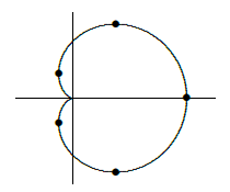
Find the points at which the curve given by $r=1+\cos\theta$ has a vertical or horizontal tangent line. Since this function has period $2\pi$, we may restrict our attention to the interval $[0,2\pi)$ or $(-\pi,\pi]$, as convenience dictates. First, we compute the slope:

$${dy\over dx}={(1+\cos\theta)\cos\theta-\sin\theta\sin\theta\over -(1+\cos\theta)\sin\theta-\sin\theta\cos\theta}= {\cos\theta+\cos^2\theta-\sin^2\theta\over -\sin\theta-2\sin\theta\cos\theta}. \nonumber$$

This fraction is zero when the numerator is zero (and the denominator is not zero). The numerator is $2\cos^2\theta+\cos\theta-1$ so by the quadratic formula $$\cos\theta={-1\pm\sqrt{1+4\cdot2}\over 4} = -1 \quad\hbox{or}\quad {1\over 2}. \nonumber$$ This means $\theta$ is $\pi$ or $\pm \pi/3$. However, when $\theta=\pi$, the denominator is also $0$, so we cannot conclude that the tangent line is horizontal.

Setting the denominator to zero we get $$\eqalign{ -\theta-2\sin\theta\cos\theta &= 0\cr \sin\theta(1+2\cos\theta)&=0,\cr} \nonumber$$ so either $\sin\theta=0$ or $\cos\theta=-1/2$. The first is true when $\theta$ is $0$ or $\pi$, the second when $\theta) is \(2\pi/3$ or $4\pi/3$. However, as above, when $\theta=\pi$, the numerator is also $0$, so we cannot conclude that the tangent line is vertical. Figure 10.2.1 shows points corresponding to $\theta$ equal to $0$, $\pm\pi/3$, $2\pi/3$ and $4\pi/3$ on the graph of the function. Note that when $\theta=\pi$ the curve hits the origin and does not have a tangent line.

Figure 10.2.1. Points of vertical and horizontal tangency for $r=1+\cos\theta$.

We know that the second derivative $f''(x)$ is useful in describing functions, namely, in describing concavity. We can compute $f''(x)$ in terms of polar coordinates as well. We already know how to write $dy/dx=y'$ in terms of $\theta$, then

$${d\over dx}{dy\over dx}= {dy'\over dx}={dy'\over d\theta}{d\theta\over dx}={dy'/d\theta\over dx/d\theta}. \nonumber$$

The ellipsis here represents rather a substantial amount of algebra. We know from above that the cardioid has horizontal tangents at $\pm \pi/3$; substituting these values into the second derivative we get $y''(\pi/3)=-\sqrt{3}/2$ and $y''(-\pi/3)=\sqrt{3}/2$, indicating concave down and concave up respectively. This agrees with the graph of the function.

Contributors

David Guichard (Whitman College)

• Integrated by Justin Marshall.