10.4: Parametric Equations

Last updated
Save as PDF

Page ID: 514

$ \newcommand{\vecs}[1]{\overset { \scriptstyle \rightharpoonup} {\mathbf{#1}} } $

$ \newcommand{\vecd}[1]{\overset{-\!-\!\rightharpoonup}{\vphantom{a}\smash {#1}}} $

$ \newcommand{\id}{\mathrm{id}}$ $ \newcommand{\Span}{\mathrm{span}}$

( \newcommand{\kernel}{\mathrm{null}\,}\) $ \newcommand{\range}{\mathrm{range}\,}$

$ \newcommand{\RealPart}{\mathrm{Re}}$ $ \newcommand{\ImaginaryPart}{\mathrm{Im}}$

$ \newcommand{\Argument}{\mathrm{Arg}}$ $ \newcommand{\norm}[1]{\| #1 \|}$

$ \newcommand{\inner}[2]{\langle #1, #2 \rangle}$

$ \newcommand{\Span}{\mathrm{span}}$

$ \newcommand{\id}{\mathrm{id}}$

$ \newcommand{\Span}{\mathrm{span}}$

$ \newcommand{\kernel}{\mathrm{null}\,}$

$ \newcommand{\range}{\mathrm{range}\,}$

$ \newcommand{\RealPart}{\mathrm{Re}}$

$ \newcommand{\ImaginaryPart}{\mathrm{Im}}$

$ \newcommand{\Argument}{\mathrm{Arg}}$

$ \newcommand{\norm}[1]{\| #1 \|}$

$ \newcommand{\inner}[2]{\langle #1, #2 \rangle}$

$ \newcommand{\Span}{\mathrm{span}}$ $ \newcommand{\AA}{\unicode[.8,0]{x212B}}$

$ \newcommand{\vectorA}[1]{\vec{#1}} % arrow$

$ \newcommand{\vectorAt}[1]{\vec{\text{#1}}} % arrow$

$ \newcommand{\vectorB}[1]{\overset { \scriptstyle \rightharpoonup} {\mathbf{#1}} } $

$ \newcommand{\vectorC}[1]{\textbf{#1}} $

$ \newcommand{\vectorD}[1]{\overrightarrow{#1}} $

$ \newcommand{\vectorDt}[1]{\overrightarrow{\text{#1}}} $

$ \newcommand{\vectE}[1]{\overset{-\!-\!\rightharpoonup}{\vphantom{a}\smash{\mathbf {#1}}}} $

$ \newcommand{\vecs}[1]{\overset { \scriptstyle \rightharpoonup} {\mathbf{#1}} } $

$ \newcommand{\vecd}[1]{\overset{-\!-\!\rightharpoonup}{\vphantom{a}\smash {#1}}} $

$\newcommand{\avec}{\mathbf a}$ $\newcommand{\bvec}{\mathbf b}$ $\newcommand{\cvec}{\mathbf c}$ $\newcommand{\dvec}{\mathbf d}$ $\newcommand{\dtil}{\widetilde{\mathbf d}}$ $\newcommand{\evec}{\mathbf e}$ $\newcommand{\fvec}{\mathbf f}$ $\newcommand{\nvec}{\mathbf n}$ $\newcommand{\pvec}{\mathbf p}$ $\newcommand{\qvec}{\mathbf q}$ $\newcommand{\svec}{\mathbf s}$ $\newcommand{\tvec}{\mathbf t}$ $\newcommand{\uvec}{\mathbf u}$ $\newcommand{\vvec}{\mathbf v}$ $\newcommand{\wvec}{\mathbf w}$ $\newcommand{\xvec}{\mathbf x}$ $\newcommand{\yvec}{\mathbf y}$ $\newcommand{\zvec}{\mathbf z}$ $\newcommand{\rvec}{\mathbf r}$ $\newcommand{\mvec}{\mathbf m}$ $\newcommand{\zerovec}{\mathbf 0}$ $\newcommand{\onevec}{\mathbf 1}$ $\newcommand{\real}{\mathbb R}$ $\newcommand{\twovec}[2]{\left[\begin{array}{r}#1 \\ #2 \end{array}\right]}$ $\newcommand{\ctwovec}[2]{\left[\begin{array}{c}#1 \\ #2 \end{array}\right]}$ $\newcommand{\threevec}[3]{\left[\begin{array}{r}#1 \\ #2 \\ #3 \end{array}\right]}$ $\newcommand{\cthreevec}[3]{\left[\begin{array}{c}#1 \\ #2 \\ #3 \end{array}\right]}$ $\newcommand{\fourvec}[4]{\left[\begin{array}{r}#1 \\ #2 \\ #3 \\ #4 \end{array}\right]}$ $\newcommand{\cfourvec}[4]{\left[\begin{array}{c}#1 \\ #2 \\ #3 \\ #4 \end{array}\right]}$ $\newcommand{\fivevec}[5]{\left[\begin{array}{r}#1 \\ #2 \\ #3 \\ #4 \\ #5 \\ \end{array}\right]}$ $\newcommand{\cfivevec}[5]{\left[\begin{array}{c}#1 \\ #2 \\ #3 \\ #4 \\ #5 \\ \end{array}\right]}$ $\newcommand{\mattwo}[4]{\left[\begin{array}{rr}#1 \amp #2 \\ #3 \amp #4 \\ \end{array}\right]}$ $\newcommand{\laspan}[1]{\text{Span}\{#1\}}$ $\newcommand{\bcal}{\cal B}$ $\newcommand{\ccal}{\cal C}$ $\newcommand{\scal}{\cal S}$ $\newcommand{\wcal}{\cal W}$ $\newcommand{\ecal}{\cal E}$ $\newcommand{\coords}[2]{\left\{#1\right\}_{#2}}$ $\newcommand{\gray}[1]{\color{gray}{#1}}$ $\newcommand{\lgray}[1]{\color{lightgray}{#1}}$ $\newcommand{\rank}{\operatorname{rank}}$ $\newcommand{\row}{\text{Row}}$ $\newcommand{\col}{\text{Col}}$ $\renewcommand{\row}{\text{Row}}$ $\newcommand{\nul}{\text{Nul}}$ $\newcommand{\var}{\text{Var}}$ $\newcommand{\corr}{\text{corr}}$ $\newcommand{\len}[1]{\left|#1\right|}$ $\newcommand{\bbar}{\overline{\bvec}}$ $\newcommand{\bhat}{\widehat{\bvec}}$ $\newcommand{\bperp}{\bvec^\perp}$ $\newcommand{\xhat}{\widehat{\xvec}}$ $\newcommand{\vhat}{\widehat{\vvec}}$ $\newcommand{\uhat}{\widehat{\uvec}}$ $\newcommand{\what}{\widehat{\wvec}}$ $\newcommand{\Sighat}{\widehat{\Sigma}}$ $\newcommand{\lt}{<}$ $\newcommand{\gt}{>}$ $\newcommand{\amp}{&}$ $\definecolor{fillinmathshade}{gray}{0.9}$

When we computed the derivative $dy/dx$ using polar coordinates, we used the expressions $x=f(\theta)\cos\theta$ and $y=f(\theta)\sin\theta$. These two equations completely specify the curve, though the form $r=f(\theta)$ is simpler. The expanded form has the virtue that it can easily be generalized to describe a wider range of curves than can be specified in rectangular or polar coordinates.

Suppose $f(t)$ and $g(t)$ are functions. Then the equations $x=f(t)$ and $y=g(t)$ describe a curve in the plane. In the case of the polar coordinates equations, the variable $t$ is replaced by $\theta$ which has a natural geometric interpretation. But $t$ in general is simply an arbitrary variable, often called in this case a parameter, and this method of specifying a curve is known as parametric equations. One important interpretation of $t$ is time. In this interpretation, the equations $x=f(t)$ and $y=g(t)$ give the position of an object at time $t$.

Example 10.4.1

Describe the path of an object that moves so that its position at time $t$ is given by$x=\cos t$, $ y=\cos^2 t$.

Solution

We see immediately that $ y=x^2$, so the path lies on this parabola. The path is not the entire parabola, however, since $x=\cos t$ is always between$-1$ and $1$. It is now easy to see that the object oscillates back and forth on the parabola between the endpoints $(1,1)$ and $(-1,1)$, and is at point $(1,1)$ at time $t=0$.

It is sometimes quite easy to describe a complicated path in parametric equations when rectangular and polar coordinate expressions are difficult or impossible to devise.

Example 10.4.2

A wheel of radius 1 rolls along a straight line, say the $x$-axis. A point on the rim of the wheel will trace out a curve, called a cycloid. Assume the point starts at the origin; find parametric equations for the curve.

Solution

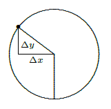
Figure 10.4.1 illustrates the generation of the curve (click on the AP link to see an animation). The wheel is shown at its starting point, and again after it has rolled through about 490 degrees. We take as our parameter $t$ the angle through which the wheel has turned, measured as shown clockwise from the line connecting the center of the wheel to the ground. Because the radius is 1, the center of the wheel has coordinates$(t,1)$. We seek to write the coordinates of the point on the rim as $(t+\Delta x,1+\Delta y)$, where $\Delta x$ and $\Delta y$ are as shown in figure 10.4.2. These values are nearly the sine and cosine of the angle$t$, from the unit circle definition of sine and cosine. However, some care is required because we are measuring$t$from a nonstandard starting line and in a clockwise direction, as opposed to the usual counterclockwise direction. A bit of thought reveals that $\Delta x=-\sin t$ and $\Delta y=-\cos t$. Thus the parametric equations for the cycloid are $x=t-\sin t$, $y=1-\cos t$.

$alt$

Figure 10.4.1. A cycloid.

$alt$

Figure 10.4.2. The wheel.

Contributors

David Guichard (Whitman College)
Integrated by Justin Marshall.

Search

Text Color

Text Size

Margin Size

Font Type