3.4: Graph Using the y-Intercept and Slope
- Page ID
- 18343
\( \newcommand{\vecs}[1]{\overset { \scriptstyle \rightharpoonup} {\mathbf{#1}} } \)
\( \newcommand{\vecd}[1]{\overset{-\!-\!\rightharpoonup}{\vphantom{a}\smash {#1}}} \)
\( \newcommand{\dsum}{\displaystyle\sum\limits} \)
\( \newcommand{\dint}{\displaystyle\int\limits} \)
\( \newcommand{\dlim}{\displaystyle\lim\limits} \)
\( \newcommand{\id}{\mathrm{id}}\) \( \newcommand{\Span}{\mathrm{span}}\)
( \newcommand{\kernel}{\mathrm{null}\,}\) \( \newcommand{\range}{\mathrm{range}\,}\)
\( \newcommand{\RealPart}{\mathrm{Re}}\) \( \newcommand{\ImaginaryPart}{\mathrm{Im}}\)
\( \newcommand{\Argument}{\mathrm{Arg}}\) \( \newcommand{\norm}[1]{\| #1 \|}\)
\( \newcommand{\inner}[2]{\langle #1, #2 \rangle}\)
\( \newcommand{\Span}{\mathrm{span}}\)
\( \newcommand{\id}{\mathrm{id}}\)
\( \newcommand{\Span}{\mathrm{span}}\)
\( \newcommand{\kernel}{\mathrm{null}\,}\)
\( \newcommand{\range}{\mathrm{range}\,}\)
\( \newcommand{\RealPart}{\mathrm{Re}}\)
\( \newcommand{\ImaginaryPart}{\mathrm{Im}}\)
\( \newcommand{\Argument}{\mathrm{Arg}}\)
\( \newcommand{\norm}[1]{\| #1 \|}\)
\( \newcommand{\inner}[2]{\langle #1, #2 \rangle}\)
\( \newcommand{\Span}{\mathrm{span}}\) \( \newcommand{\AA}{\unicode[.8,0]{x212B}}\)
\( \newcommand{\vectorA}[1]{\vec{#1}} % arrow\)
\( \newcommand{\vectorAt}[1]{\vec{\text{#1}}} % arrow\)
\( \newcommand{\vectorB}[1]{\overset { \scriptstyle \rightharpoonup} {\mathbf{#1}} } \)
\( \newcommand{\vectorC}[1]{\textbf{#1}} \)
\( \newcommand{\vectorD}[1]{\overrightarrow{#1}} \)
\( \newcommand{\vectorDt}[1]{\overrightarrow{\text{#1}}} \)
\( \newcommand{\vectE}[1]{\overset{-\!-\!\rightharpoonup}{\vphantom{a}\smash{\mathbf {#1}}}} \)
\( \newcommand{\vecs}[1]{\overset { \scriptstyle \rightharpoonup} {\mathbf{#1}} } \)
\(\newcommand{\longvect}{\overrightarrow}\)
\( \newcommand{\vecd}[1]{\overset{-\!-\!\rightharpoonup}{\vphantom{a}\smash {#1}}} \)
\(\newcommand{\avec}{\mathbf a}\) \(\newcommand{\bvec}{\mathbf b}\) \(\newcommand{\cvec}{\mathbf c}\) \(\newcommand{\dvec}{\mathbf d}\) \(\newcommand{\dtil}{\widetilde{\mathbf d}}\) \(\newcommand{\evec}{\mathbf e}\) \(\newcommand{\fvec}{\mathbf f}\) \(\newcommand{\nvec}{\mathbf n}\) \(\newcommand{\pvec}{\mathbf p}\) \(\newcommand{\qvec}{\mathbf q}\) \(\newcommand{\svec}{\mathbf s}\) \(\newcommand{\tvec}{\mathbf t}\) \(\newcommand{\uvec}{\mathbf u}\) \(\newcommand{\vvec}{\mathbf v}\) \(\newcommand{\wvec}{\mathbf w}\) \(\newcommand{\xvec}{\mathbf x}\) \(\newcommand{\yvec}{\mathbf y}\) \(\newcommand{\zvec}{\mathbf z}\) \(\newcommand{\rvec}{\mathbf r}\) \(\newcommand{\mvec}{\mathbf m}\) \(\newcommand{\zerovec}{\mathbf 0}\) \(\newcommand{\onevec}{\mathbf 1}\) \(\newcommand{\real}{\mathbb R}\) \(\newcommand{\twovec}[2]{\left[\begin{array}{r}#1 \\ #2 \end{array}\right]}\) \(\newcommand{\ctwovec}[2]{\left[\begin{array}{c}#1 \\ #2 \end{array}\right]}\) \(\newcommand{\threevec}[3]{\left[\begin{array}{r}#1 \\ #2 \\ #3 \end{array}\right]}\) \(\newcommand{\cthreevec}[3]{\left[\begin{array}{c}#1 \\ #2 \\ #3 \end{array}\right]}\) \(\newcommand{\fourvec}[4]{\left[\begin{array}{r}#1 \\ #2 \\ #3 \\ #4 \end{array}\right]}\) \(\newcommand{\cfourvec}[4]{\left[\begin{array}{c}#1 \\ #2 \\ #3 \\ #4 \end{array}\right]}\) \(\newcommand{\fivevec}[5]{\left[\begin{array}{r}#1 \\ #2 \\ #3 \\ #4 \\ #5 \\ \end{array}\right]}\) \(\newcommand{\cfivevec}[5]{\left[\begin{array}{c}#1 \\ #2 \\ #3 \\ #4 \\ #5 \\ \end{array}\right]}\) \(\newcommand{\mattwo}[4]{\left[\begin{array}{rr}#1 \amp #2 \\ #3 \amp #4 \\ \end{array}\right]}\) \(\newcommand{\laspan}[1]{\text{Span}\{#1\}}\) \(\newcommand{\bcal}{\cal B}\) \(\newcommand{\ccal}{\cal C}\) \(\newcommand{\scal}{\cal S}\) \(\newcommand{\wcal}{\cal W}\) \(\newcommand{\ecal}{\cal E}\) \(\newcommand{\coords}[2]{\left\{#1\right\}_{#2}}\) \(\newcommand{\gray}[1]{\color{gray}{#1}}\) \(\newcommand{\lgray}[1]{\color{lightgray}{#1}}\) \(\newcommand{\rank}{\operatorname{rank}}\) \(\newcommand{\row}{\text{Row}}\) \(\newcommand{\col}{\text{Col}}\) \(\renewcommand{\row}{\text{Row}}\) \(\newcommand{\nul}{\text{Nul}}\) \(\newcommand{\var}{\text{Var}}\) \(\newcommand{\corr}{\text{corr}}\) \(\newcommand{\len}[1]{\left|#1\right|}\) \(\newcommand{\bbar}{\overline{\bvec}}\) \(\newcommand{\bhat}{\widehat{\bvec}}\) \(\newcommand{\bperp}{\bvec^\perp}\) \(\newcommand{\xhat}{\widehat{\xvec}}\) \(\newcommand{\vhat}{\widehat{\vvec}}\) \(\newcommand{\uhat}{\widehat{\uvec}}\) \(\newcommand{\what}{\widehat{\wvec}}\) \(\newcommand{\Sighat}{\widehat{\Sigma}}\) \(\newcommand{\lt}{<}\) \(\newcommand{\gt}{>}\) \(\newcommand{\amp}{&}\) \(\definecolor{fillinmathshade}{gray}{0.9}\)- Identify and find the slope of a line.
- Graph a line using the slope and \(y\)-intercept.
Slope
The steepness of any incline can be measured as the ratio of the vertical change to the horizontal change. For example, a \(5\)% incline can be written as \(\frac{5}{100}\), which means that for every \(100\) feet forward, the height increases \(5\) feet.
.png?revision=1)
Figure \(\PageIndex{1}\)
In mathematics, we call the incline of a line the slope and use the letter \(m\) to denote it. The vertical change is called the rise and the horizontal change is called the run.
\[\color{Cerulean}{Slope}\quad\color{black}{m=\frac{\text{vertical change}}{\text{horizontal change}}=\frac{rise}{run}}\]
The rise and the run can be positive or negative. A positive rise corresponds to a vertical change up and a negative rise corresponds to a vertical change down. A positive run denotes a horizontal change to the right and a negative run corresponds to a horizontal change to the left. Given the graph, we can calculate the slope by determining the vertical and horizontal changes between any two points.
Find the slope of the given line:
.png?revision=1)
Figure \(\PageIndex{2}\)
Solution:
From the given points on the graph, count \(3\) units down and \(4\) units right.
\(m=\frac{rise}{run}=\frac{-3\:\text{units}}{4\:\text{units}}=-\frac{3}{4}\)
Answer:
\(m=-\frac{3}{4}\)
Here we have a negative slope, which means that for every \(4\) units of movement to the right, the vertical change is \(3\) units downward. There are four geometric cases for the value of the slope.
.png?revision=1)
Figure \(\PageIndex{3}\)
Reading the graph from left to right, we see that lines with an upward incline have positive slopes and lines with a downward incline have negative slopes.
.png?revision=1)
Figure \(\PageIndex{4}\)
If the line is horizontal, then the rise is \(0\):
\(m=\frac{rise}{run}=\frac{0}{run}=0\)
The slope of a horizontal line is \(0\). If the line is vertical, then the run is \(0\):
\(m=\frac{rise}{run}=\frac{rise}{0}\quad\color{Cerulean}{Undefined}\)
The slope of a vertical line is undefined.
Find the slope of the given line:
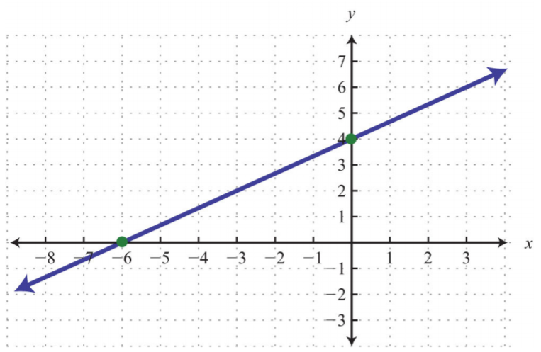.png?revision=1)
Figure \(\PageIndex{5}\)
- Answer
-
\(m=\frac{2}{3}\)
Calculating the slope can be difficult if the graph does not have points with integer coordinates. Therefore, we next develop a formula that allows us to calculate the slope algebraically. Given any two points \((x_{1}, y_{1})\) and \((x_{2}, y_{2})\), we can obtain the rise and run by subtracting the corresponding coordinates.
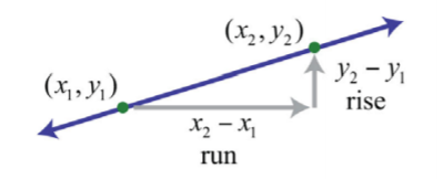.png?revision=1)
Figure \(\PageIndex{6}\)
This leads us to the slope formula. Given any two points \((x_{1}, y_{1})\) and \((x_{2}, y_{2})\), the slope is given by
\(m=\frac{rise}{run}=\frac{y_{2}-y_{1}}{x_{2}-x_{1}}\)
Find the slope of the line passing through \((−3, −5)\) and \((2, 1)\).
Solution:
Given \((−3, −5)\) and \((2, 1)\), calculate the difference of the \(y\)-values divided by the difference of the \(x\)-values. Since subtraction is not commutative, take care to be consistent when subtracting the coordinates.
\(\begin{array}{cc}{(x_{1},y_{1})}&{(x_{2},y_{2})}\\{(-3,-5)}&{(2,1)}\end{array}\)
\(\begin{aligned} m&=\frac{y_{2}-y_{1}}{x_{2}-x_{1}} \\ &=\frac{1-(-5)}{2-(-3)} \\ &=\frac{1+5}{2+3} \\ &=\frac{6}{5} \end{aligned}\)
Answer:
\(m=\frac{6}{5}\)
We can graph the line described in the previous example and verify that the slope is \(\frac{6}{5}\).
.png?revision=1)
Figure \(\PageIndex{7}\)
Certainly the graph is optional; the beauty of the slope formula is that we can obtain the slope, given two points, using only algebra.
Find the slope of the line passing through \((−4, 3)\) and \((−1, −7)\).
Solution:
\(\begin{array}{cc}{(x_{1},y_{1})}&{(x_{2},y_{2})}\\{(-4,3)}&{(-1,-7)} \end{array}\)
\(m=\frac{y_{2}-y_{1}}{x_{2}-x_{1}}=\frac{-7-(3)}{-1-(-4)}=\frac{-7-3}{-1+4}=\frac{-10}{3}\)
Answer:
\(m=-\frac{10}{3}\)
When using the slope formula, take care to be consistent since order does matter. You must subtract the coordinates of the first point from the coordinates of the second point for both the numerator and the denominator in the same order.
Find the slope of the line passing through \((7, −2)\) and \((−5, −2)\).
Solution:
\(\begin{array}{cc}{(x_{1},y_{1})}&{(x_{2},y_{2})}\\{(7,-2)}&{(-5,-2)} \end{array}\)
\(m=\frac{y_{2}-y_{1}}{x_{2}-x_{1}}=\frac{-2-(-2)}{-5-(7)}=\frac{-2+2}{-5-7}=\frac{0}{-12}=0\)
Answer:
\(m=0\). As an exercise, plot the given two points and verify that they lie on a horizontal line.
Find the slope of the line passing through \((−4, −3)\) and \((−4, 5)\).
Solution:
\(\begin{array}{cc}{(x_{1},y_{1})}&{(x_{2},y_{2})}\\{(-4,-3)}&{(-4,5)} \end{array}\)
\(m=\frac{y_{2}-y_{1}}{x_{2}-x_{1}}=\frac{5-(-3)}{-4-(-4)}=\frac{5+3}{-4+4}=\frac{8}{0}\quad\color{Cerulean}{Undefined}\)
Answer:
The slope \(m\) is undefined. As an exercise, plot the given two points and verify that they lie on a vertical line.
Calculate the slope of the line passing through \((−2, 3)\) and \((5, −5)\).
- Answer
-
\(m=-\frac{8}{7}\)
When considering the slope as a rate of change it is important to include the correct units.
A Corvette Coupe was purchased new in 1970 for about $\(5,200\) and depreciated in value over time until it was sold in 1985 for $\(1,300\). At this point, the car was beginning to be considered a classic and started to increase in value. In the year 2000, when the car was 30 years old, it sold at auction for $\(10,450\). The following line graph depicts the value of the car over time.
.png?revision=1)
Figure \(\PageIndex{8}\)
- Determine the rate at which the car depreciated in value from 1970 to 1985.
- Determine the rate at which the car appreciated in value from 1985 to 2000.
Solution:
Notice that the value depends on the age of the car and that the slope measures the rate in dollars per year.
a. The slope of the line segment depicting the value for the first 15 years is
\(m=\frac{y_{2}-y_{1}}{x_{2}-x_{1}}=\frac{$1,300-$5,200}{15\text{ years}-0\text{ years}}=\frac{-$3,900}{15\text{ years}}=-$260\text{ per year}\)
b. The slope of the line segment depicting the value for the next 15 years is
\(m=\frac{y_{2}-y_{1}}{x_{2}-x_{1}}=\frac{$10,450-$1,300}{30\text{ years}-15\text{ years}}=\frac{$9,150}{15\text{ years}}=$610\text{ per year}\)
Answer:
- The value of the car depreciated $\(260\) per year from 1970 to 1985.
- The value of the car appreciated $\(610\) per year from 1985 to 2000.
Slope-Intercept Form of a Line
To this point, we have learned how to graph lines by plotting points and by using the \(x\)- and \(y\)-intercepts. In addition, we have seen that we need only two points to graph a line. In this section, we outline a process to easily determine two points using the \(y\)-intercept and the slope. The equation of any nonvertical line can be written in slope-intercept form \(y=mx+b\). In this form, we can identify the slope, \(m\), and the \(y\)-intercept, \((0, b)\).
Determine the slope and \(y\)-intercept:
\(y=−\frac{4}{5}x+7\).
Solution:
In this form, the coefficient of \(x\) is the slope, and the constant is the \(y\)-value of the \(y\)-intercept. Therefore, by inspection, we have
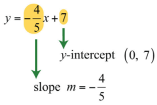.png?revision=1)
Figure \(\PageIndex{9}\)
Answer:
The \(y\)-intercept is \((0, 7)\), and the slope is \(m=−\frac{4}{5}\).
It is not always the case that the linear equation is given in slope-intercept form. When it is given in standard form, you have to first solve for \(y\) to obtain slope-intercept form.
Express \(3x+5y=30\) in slope-intercept form and then identify the slope and \(y\)-intercept.
Solution:
Begin by solving for \(y\). To do this, apply the properties of equality to first isolate \(5y\) and then divide both sides by \(5\).
\(\begin{aligned} 3x+5y&=30 \\ 3x+5y\color{Cerulean}{-3x}&=30\color{Cerulean}{-3x} \\ 5y&=-3x+30 \\ \frac{5y}{\color{Cerulean}{5}}&=\frac{-3x+30}{\color{Cerulean}{5}} \\ y&=\frac{-3x}{5}+\frac{30}{5} \\ y&=-\frac{3}{5}x+6 \end{aligned}\)
Answer:
Slope-intercept form: \(y=−\frac{3}{5}x+6\); \(y\)-intercept: \((0, 6)\); slope: \(m=−\frac{3}{5}\)
Once the equation is in slope-intercept form, we immediately have one point to plot, the \(y\)-intercept. From the intercept, you can mark off the slope to plot another point on the line. From the previous example we have
\(y=-\frac{3}{5}x+6\)
\(y\)-intercept: \((0,6)\)
slope: \(m=-\frac{3}{5}=\frac{-3}{5}=\frac{rise}{run}\)
Starting from the point \((0, 6)\), use the slope to mark another point \(3\) units down and \(5\) units to the right.
.png?revision=1)
Figure \(\PageIndex{10}\)
It is not necessary to check that the second point, (5, 3), solves the original linear equation. However, we do it here for the sake of completeness.
\(\begin{aligned} 3x+5y&=30 \\ 3(\color{OliveGreen}{5}\color{black}{)+5(}\color{OliveGreen}{3}\color{black}{)}&=30 \\ 15+15&=30 \\ 30&=30\quad\color{Cerulean}{\checkmark} \end{aligned}\)
Marking off the slope in this fashion produces as many ordered pair solutions as we desire. Notice that if we mark off the slope again, from the point \((5, 3)\), then we obtain the \(x\)-intercept, \((10, 0)\).
Graph:
\(−x+2y=4\).
Solution:
In this example, we outline the general steps for graphing a line using slope-intercept form.
Step 1: Solve for \(y\) to obtain slope-intercept form.
\(\begin{aligned} -x+2y&=4 \\ -x+2y\color{Cerulean}{+x}&=4\color{Cerulean}{+x} \\ 2y&=x+4 \\ \frac{2y}{\color{Cerulean}{2}}&=\frac{x+4}{\color{Cerulean}{2}} \\ y&=\frac{1x}{2}+\frac{4}{2} \\ y&=\frac{1}{2}x+2 \end{aligned}\)
Step 2: Identify the \(y\)-intercept and slope.
\(y\)-intercept: \((0,2)\)
slope: \(m=\frac{1}{2}=\frac{rise}{run}\)
Step 3: Plot the \(y\)-intercept and use the slope to find another ordered pair solution. Starting from the \(y\)-intercept, mark off the slope and identify a second point. In this case, mark a point after a rise of \(1\) unit and a run of \(2\) units.
.png?revision=1)
Figure \(\PageIndex{11}\)
Step 4: Draw the line through the two points with a straightedge.
Answer:
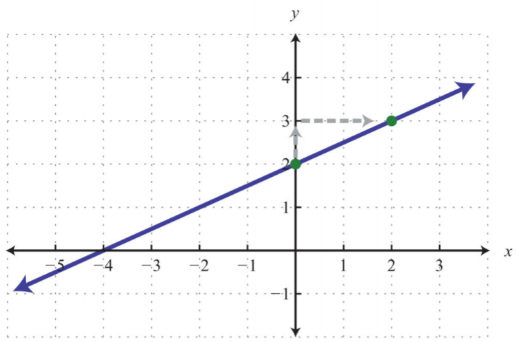.png?revision=1)
Figure \(\PageIndex{12}\)
In this example, we notice that we could get the \(x\)-intercept by marking off the slope in a different but equivalent manner. Consider the slope as the ratio of two negative numbers as follows:
\(m=\frac{1}{2}=\frac{-1}{-2}=\frac{rise}{run}\)
We could obtain another point on the line by marking off the equivalent slope down \(1\) unit and left \(2\) units. We do this twice to obtain the \(x\)-intercept, \((−4, 0)\).
.png?revision=1)
Figure \(\PageIndex{13}\)
Marking off the slope multiple times is not necessarily always going to give us the \(x\)-intercept, but when it does, we obtain a valuable point with little effort. In fact, it is a good practice to mark off the slope multiple times; doing so allows you to obtain more points on the line and produce a more accurate graph.
Graph and find the \(x\)-intercept:
\(y=\frac{3}{4}x−2\).
Solution:
The equation is given in slope-intercept form. Therefore, by inspection, we have the \(y\)-intercept and slope.
\(y\)-intercept: \((0,-2)\)
slope: \(m=\frac{3}{4}=\frac{rise}{run}\)
.png?revision=1)
Figure \(\PageIndex{14}\)
We can see that the \(x\)-value of the \(x\)-intercept is a mixed number between \(2\) and \(3\). To algebraically find \(x\)-intercepts, recall that we must set \(y = 0\) and solve for \(x\).
Answer:
The \(x\)-intercept is \((2\frac{2}{3}, 0)\).
Graph:
\(x−y=0\).
Solution:
Begin by solving for \(y\).
\(\begin{aligned} x-y&=0\\x-y\color{Cerulean}{-x}&=0\color{Cerulean}{-x} \\ -y&=-x \\ \color{Cerulean}{-1\cdot}\color{black}{(-y)}&=\color{Cerulean}{-1\cdot}\color{black}{(-x)} \\ y&=x \end{aligned}\)
The equation \(y=x\) can be written \(y=1x+0\), and we have
\(y\)-intercept: \((0,0)\)
slope: \(m=1=\frac{1}{1}=\frac{rise}{run}\)
Answer:
.png?revision=1)
Figure \(\PageIndex{15}\)
Graph \(−2x+5y=20\) and label the \(x\)-intercept.
- Answer
-
.png?revision=1)
Figure \(\PageIndex{16}\)
Key Takeaways
- Slope measures the steepness of a line as rise over run. A positive rise denotes a vertical change up, and a negative rise denotes a vertical change down. A positive run denotes a horizontal change right, and a negative run denotes a horizontal change left.
- Horizontal lines have a slope of zero, and vertical lines have undefined slopes.
- Given any two points on a line, we can algebraically calculate the slope using the slope formula, \(m=\frac{rise}{run}=\frac{y_{2}−y_{1}}{x_{2}−x_{1}}\).
- Any nonvertical line can be written in slope-intercept form, \(y=mx+b\), from which we can determine, by inspection, the slope \(m\) and \(y\)-intercept \((0, b)\).
- If we know the \(y\)-intercept and slope of a line, then we can easily graph it. First, plot the \(y\)-intercept, and from this point use the slope as rise over run to mark another point on the line. Finally, draw a line through these two points with a straightedge and add an arrow on either end to indicate that it extends indefinitely.
- We can obtain as many points on the line as we wish by marking off the slope multiple times.
Determine the slope and the \(y\)-intercept of the given graph.
1.
.png?revision=1)
Figure \(\PageIndex{17}\)
2.
.png?revision=1)
Figure \(\PageIndex{18}\)
3.
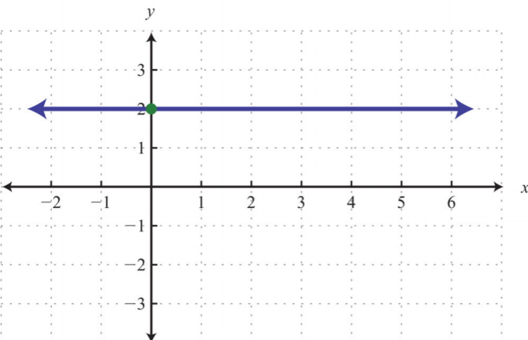.png?revision=1)
Figure \(\PageIndex{19}\)
4.
.png?revision=1)
Figure \(\PageIndex{20}\)
5.
.png?revision=1)
Figure \(\PageIndex{21}\)
6.
.png?revision=1)
Figure \(\PageIndex{22}\)
- Answer
-
1. \(y\)-intercept: \((0, 3)\); slope: \(m = −\frac{3}{4}\)
3. \(y\)-intercept: \((0, 2)\); slope: \(m = 0\)
5. \(y\)-intercept: \((0, 0)\); slope: \(m = 2\)
Determine the slope, given two points.
- \((3, 2)\) and \((5, 1)\)
- \((7, 8)\) and \((−3, 5)\)
- \((2, −3)\) and \((−3, 2)\)
- \((−3, 5)\) and \((7, −5)\)
- \((−1, −6)\) and \((3, 2)\)
- \((5, 3)\) and \((4, 12)\)
- \((−9, 3)\) and \((−6, −5)\)
- \((−22, 4)\) and \((−8, −12)\)
- \((\frac{1}{2}, −\frac{1}{3})\) and \((−\frac{1}{2}, \frac{2}{3})\)
- \((−\frac{3}{4}, \frac{3}{2})\) and \((\frac{1}{4}, −\frac{1}{2})\)
- \((−\frac{1}{3}, \frac{5}{8})\) and \((\frac{1}{2}, −\frac{3}{4})\)
- \((−\frac{3}{5}, −\frac{3}{2})\) and \((\frac{1}{10}, \frac{4}{5})\)
- \((3, −5)\) and \((5, −5)\)
- \((−3, 1)\) and \((−14, 1)\)
- \((−2, 3)\) and \((−2, −4)\)
- \((−4, −4)\) and \((5, 5)\)
- A roof drops \(4\) feet for every \(12\) feet forward. Determine the slope of the roof.
- A road drops \(300\) feet for every \(5,280\) feet forward. Determine the slope of the road.
- The following graph gives the US population of persons 65 years old and over. At what rate did this population increase from 2000 to 2008?
.png?revision=1)
Figure \(\PageIndex{23}\): Source: US Census Bureau.
20. The following graph gives total consumer credit outstanding in the United States. At what rate did consumer credit increase from 2002 to 2008?
.png?revision=1)
Figure \(\PageIndex{24}\): Source: US Census Bureau.
21. A commercial van was purchased new for $\(20,000\) and is expected to be worth $\(4,000\) in 8 years. Determine the rate at which the van depreciates in value.
22. A commercial-grade copy machine was purchased new for $\(4,800\) and will be considered worthless in 6 years. Determine the rate at which the copy machine depreciates in value.
23. Find \(y\) if the slope of the line passing through \((−2, 3)\) and \((4, y)\) is \(12\).
24. Find \(y\) if the slope of the line passing through \((5, y)\) and \((6, −1)\) is \(10\).
25. Find \(y\) if the slope of the line passing through \((5, y)\) and \((−4, 2)\) is \(0\).
26. Find \(x\) if the slope of the line passing through \((−3, 2)\) and \((x, 5)\) is undefined.
- Answer
-
1. \(−\frac{1}{2}\)
3. \(−1\)
5. \(2\)
7. \(−\frac{8}{3}\)
9. \(−1\)
11. \(−\frac{33}{20}\)
13. \(0\)
15. Undefined
17. \(−\frac{1}{3}\)
19. \(\frac{1}{2}\) million per year
21. $\(2,000\) per year
23. \(75\)
25. \(2\)
Express the given linear equation in slope-intercept form and identify the slope and \(y\)-intercept.
- \(6x−5y=30\)
- \(−2x+7y=28\)
- \(9x−y=17\)
- \(x−3y=18\)
- \(2x−3y=0\)
- \(−6x+3y=0\)
- \(\frac{2}{3}x−\frac{5}{4}y=10\)
- \(−\frac{4}{3}x+\frac{1}{5}y=−5\)
- Answer
-
1. \(y=\frac{6}{5}x−6\); slope: \(\frac{6}{5}\); \(y\)-intercept: \((0, −6)\)
3. \(y=9x−17\); slope: \(9\); \(y\)-intercept: \((0, −17)\)
5. \(y=\frac{2}{3}x\); slope: \(\frac{2}{3}\); \(y\)-intercept: \((0, 0)\)
7. \(y=\frac{8}{15}x−8\); slope: \(\frac{8}{15}\); \(y\)-intercept: \((0, −8)\)
Graph the line given the slope and the \(y\)-intercept.
- \(m=\frac{1}{3}\) and \((0, −2)\)
- \(m=−\frac{2}{3}\) and \((0, 4)\)
- \(m=3\) and \((0, 1)\)
- \(m=−2\) and \((0, −1)\)
- \(m=0\) and \((0, 5)\)
- \(m\) undefined and \((0, 0)\)
- \(m=1\) and \((0, 0)\)
- \(m=−1\) and \((0, 0)\)
- \(m=−\frac{15}{3}\) and \((0, 20)\)
- \(m=−10\) and \((0, −5)\)
- Answer
-
1.
.png?revision=2)
Figure \(\PageIndex{25}\)
3.
.png?revision=1)
Figure \(\PageIndex{26}\)
5.
.png?revision=1)
Figure \(\PageIndex{27}\)
7.
.png?revision=1)
Figure \(\PageIndex{28}\)
9.
.png?revision=1)
Figure \(\PageIndex{29}\)
Graph using the slope and \(y\)-intercept.
- \(y=\frac{2}{3}x−2\)
- \(y=−\frac{1}{3}x+1\)
- \(y=−3x+6\)
- \(y=3x+1\)
- \(y=\frac{3}{5}x\)
- \(y=−\frac{3}{7}x\)
- \(y=−8\)
- \(y=7\)
- \(y=−x+2\)
- \(y=x+1\)
- \(y=\frac{1}{2}x+\frac{3}{2}\)
- \(y=−\frac{3}{4}x+\frac{5}{2}\)
- \(4x+y=7\)
- \(3x−y=5\)
- \(5x−2y=10\)
- \(−2x+3y=18\)
- \(x−y=0\)
- \(x+y=0\)
- \(\frac{1}{2}x−\frac{1}{3}y=1\)
- \(−\frac{2}{3}x+\frac{1}{2}y=2\)
- \(3x+2y=1\)
- \(5x+3y=1\)
- On the same set of axes, graph the three lines, where \(y=\frac{3}{2}x+b\) and \(b = \{−2, 0, 2\}\).
- On the same set of axes, graph the three lines, where \(y=mx+1\) and \(m = \{−\frac{1}{2}, 0, \frac{1}{2}\}\).
- Answer
-
1.
.png?revision=1)
Figure \(\PageIndex{30}\)
3.
.png?revision=1)
Figure \(\PageIndex{31}\)
5.
.png?revision=1)
Figure \(\PageIndex{32}\)
7.
.png?revision=1)
Figure \(\PageIndex{33}\)
9.
.png?revision=1)
Figure \(\PageIndex{34}\)
11.
.png?revision=1)
Figure \(\PageIndex{35}\)
13.
.png?revision=1)
Figure \(\PageIndex{36}\)
15.
.png?revision=1)
Figure \(\PageIndex{37}\)
17.
.png?revision=1)
Figure \(\PageIndex{38}\)
19.
.png?revision=1)
Figure \(\PageIndex{39}\)
21.
.png?revision=1)
Figure \(\PageIndex{40}\)
23.
.png?revision=1)
Figure \(\PageIndex{41}\)
- Name three methods for graphing lines. Discuss the pros and cons of each method.
- Choose a linear equation and graph it three different ways. Scan the work and share it on the discussion board.
- Why do we use the letter m for slope?
- How are equivalent fractions useful when working with slopes?
- Can we graph a line knowing only its slope?
- Research and discuss the alternative notation for slope: \(m=\frac{Δy}{Δx}\).
- What strategies for graphing lines should be brought to an exam? Explain
- Answer
-
1. Answers may vary
3. Answers may vary
5. Answers may vary
7. Answers may vary


