1.27: Rectangular Coordinate System

Last updated
Save as PDF

Page ID: 48445

$ \newcommand{\vecs}[1]{\overset { \scriptstyle \rightharpoonup} {\mathbf{#1}} } $ $ \newcommand{\vecd}[1]{\overset{-\!-\!\rightharpoonup}{\vphantom{a}\smash {#1}}} $$\newcommand{\id}{\mathrm{id}}$ $ \newcommand{\Span}{\mathrm{span}}$ $ \newcommand{\kernel}{\mathrm{null}\,}$ $ \newcommand{\range}{\mathrm{range}\,}$ $ \newcommand{\RealPart}{\mathrm{Re}}$ $ \newcommand{\ImaginaryPart}{\mathrm{Im}}$ $ \newcommand{\Argument}{\mathrm{Arg}}$ $ \newcommand{\norm}[1]{\| #1 \|}$ $ \newcommand{\inner}[2]{\langle #1, #2 \rangle}$ $ \newcommand{\Span}{\mathrm{span}}$ $\newcommand{\id}{\mathrm{id}}$ $ \newcommand{\Span}{\mathrm{span}}$ $ \newcommand{\kernel}{\mathrm{null}\,}$ $ \newcommand{\range}{\mathrm{range}\,}$ $ \newcommand{\RealPart}{\mathrm{Re}}$ $ \newcommand{\ImaginaryPart}{\mathrm{Im}}$ $ \newcommand{\Argument}{\mathrm{Arg}}$ $ \newcommand{\norm}[1]{\| #1 \|}$ $ \newcommand{\inner}[2]{\langle #1, #2 \rangle}$ $ \newcommand{\Span}{\mathrm{span}}$$\newcommand{\AA}{\unicode[.8,0]{x212B}}$

In Chapter 1, we learned that a real number can be represented as a point on a number line. In this section we will learn that an ordered pair of real numbers can be represented as a point in a plane. This plane is called a rectangular coordinate system or Cartesian coordinate system named after a French mathematician, Ren´e Descartes.

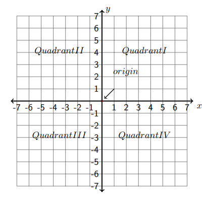
The figure on the next page shows the rectangular coordinate system. It consists of two number lines perpendicular to each other. The horizontal line is called x-axis, and the vertical line is called $y$-axis. The two number lines intersect at the origin of each number line and the intersection is called the origin of the coordinate system. The axes divide the plane into four regions. They are called quadrants. From the top right to the bottom right, the quadrants are ordered as I, II, III and IV in a counter-clockwise direction.

Every point $P$ on the plane is represented by an ordered pair $(x, y),$ which is referred to as the coordinates of the point $P$. The first value is called $x$ coordinate, and the second one is called $y$ -coordinate. The $x$ -coordinate measures the distance of the point from the $y$ -axis, and the $y$ -coordinate measures the distance of the point from the $x$ -axis. If $x>0,$ the point is to the right of the $y$ -axis; if $x<0,$ the point is to the left of the $y$ -axis; if $x=0,$ the point is on the $y$ -axis. If $y>0,$ the point is above the $x$ -axis; if $y<0,$ the point is below the $y$ -axis; if $y=0,$ the point is on the $x$ -axis.

$clipboard_e2e2406031be20f6e61740ad0fc8eed78.png$

Example 25.1

Plot the given points on the rectangular coordinate system.

(A) $(4, 2)$, (B) $(−2, 3)$, (C) $(−3, −1)$, (D) $(2, −4)$ (E) $(0, 1)$, (F) $(−1, 0)$

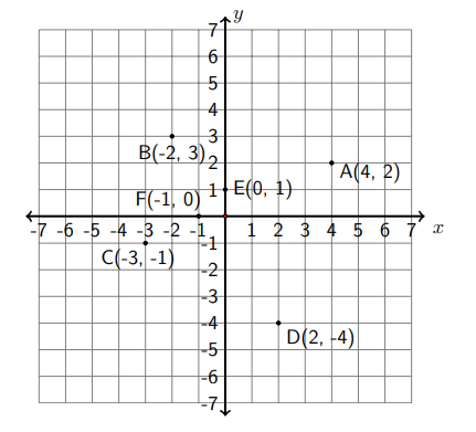
$clipboard_e9a6e5039e1b8dbb92934419f84d7ba81.png$

To plot point $(4,2),$ we start from the origin then move 4 units to the right and 2 units up. The point (4,2) is labeled as $A$. To plot point (-2,3) , we start from the origin then move 2 units to the left and 3 units up. The point (-2,3) is labeled as $B .$ Points $(\mathrm{C})$ and $(\mathrm{D})$ are plotted in a similar way. To plot $(0,1),$ from the origin, we only move 1 unit up, so the point $E$ is on the $y$ -axis. Similarly, the point (-1,0) is on the $x$ -axis, 1 unit to the left of the origin. The point (0,0) is just the origin of the coordinate system.

Example 25.2

Determine the coordinates of following points:

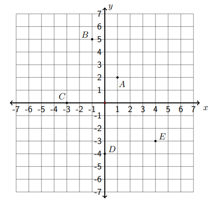
$clipboard_ed3b8116bf64e8a1fa6998851645da509.png$

Point A: 1 unit right, 2 units up $(1, 2)$

Point B: 1 unit left, 5 units up $(−1, 5)$

Point C: 3 units left, 0 units up or down (−3, 0)

Point D: 0 units left or right, 4 units down (0, −4)

Point E: 4 units right, 3 units down (4, −3)

Linear Equations in Two Variables

In Chapter 16, we solved linear equations in one variable. In this section, we will learn how to find solutions of linear equations in two variables, and how to represent them in a rectangular coordinate system.

The equation $y=2 x+3$ is an example of a linear equation in two variables, $x$ and $y$. The solution to this equation is an ordered pair of two real numbers $(a, b)$ so that when $x$ is replaced by $a$ and $y$ is replaced by $b,$ the equation is a true statement. For example, (1,5) is a solution of $y=2 x+3$ because when we substitute 1 for $x$ and 5 for $y,$ we get $5=2(1)+3,$ which is a true statement. The ordered pair (4,3) is not a solution to the equation because substituting 4 for $x$ and 3 for $y$ does not satisfy the equation i.e. $3 \neq 2(4)+3$.

Example 25.3

Check if the following ordered pairs are solutions of the equation $2 x-3 y=5$.

\[(A) (1,-1) (B) (2,1) (C) \left(\frac{5}{2}, 0\right)\nonumber\]

To check, let’s substitute the values into our equation.

(A) $2(1)-3(-1)=5 \Rightarrow 2+3=5 \Rightarrow 5=5$ True

(B) $2(2)-3(1)=5 \Rightarrow 4-3=5 \Rightarrow 1=5$ False

Therefore $(A)$ and $(C)$ are solutions and $(B)$ is not a solution.

From the last example we see that the solutions of an equation in two variables are ordered pairs $(x, y)$. Therefore they can be represented by points on a rectangular coordinate system. By connecting all possible points, we get the graph of the equation.

Now let's find the graph of the equation $y=2 x+3$ by finding solution pairs and plotting them. Since we have only one equation for two variables $x$ and $y$, we can first choose a few $x$ values, say $x=-2,-1,0,1,2,$ and then find their corresponding $y$ values. For example, if $x=-2$ then $y=2(-2)+3=-1 .$ So (-2,-1) is a solution pair. It is helpful to set up a table to keep track.

$\begin{array}{lll} \text{Value of }x & \text{Calculate }y = 2x + 3 & \text{Solution Pair}
-2 & y=2(-2)+3=-1 & (-2,-1) \\
-1 & y=2(-1)+3=1 & (-1,1) \\
0 & y=2(0)+3=3 & (0,3) \\
1 & y=2(1)+3=5 & (1,5) \\
2 & y=2(2)+3=7 & (2,7)
\end{array}$

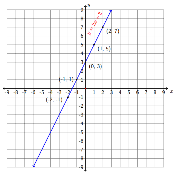
$clipboard_e691e252840d6c1ca849a4d8552805b2a.png$

After plotting these points on a rectangular coordinate system, it is easy to guess that the graph of $y=2 x+3$ might be a straight line. In fact, the graph of the equation $y=2 x+3$ is a straight line - which is why it is referred to as a linear equation.

Example 25.4

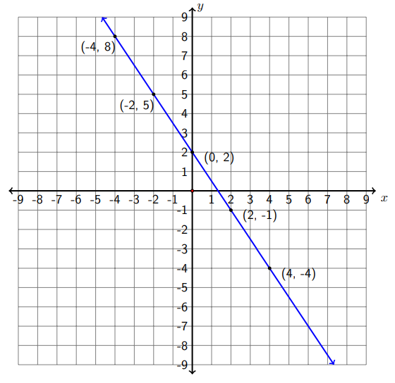
Graph the equation $3 x+2 y=4$ by plotting points.

To graph the equation, we need to first find a couple of solution pairs. Let's begin by solving for $y:$

$3 x+2 y=4 \quad \Rightarrow \quad 2 y=-3 x+4 \quad \Rightarrow \quad y=\frac{-3 x+4}{2} \quad \Rightarrow \quad y=\frac{-3 x}{2}+2$

Let $x=-4,-2,0,2,4$. Here only even numbers are chosen so the results are not fractions.

$\begin{array}{lll} \text{Value of }x & \text{Calculate }y=\frac{-3 x}{2}+2 & \text{Solution Pair}
-4 & y=\frac{-3(-4)}{2}+2=8 & (-4,8) \\
-2 & y=\frac{-3(-2)}{2}+2=5 & (-2,5) \\
0 & y=\frac{-3(0)}{2}+2=2 & (0,2) \\
2 & y=\frac{-3(2)}{2}+2=-1 & (2,-1) \\
4 & y=\frac{-3(4)}{2}+2=-4 & (4,-4)
\end{array}$

The graph of the line $3 x+2 y=4$ is shown in the following figure.

$clipboard_e32bb44a80ac3538c31502cf424e4b372.png$

Exit Problem

Graph the equation: $3 x+2 y=8$