1.30: Solving a System of Equations Graphically

Last updated
Save as PDF

Page ID: 41231

Samar ElHitti, Marianna Bonanome, Holly Carley, Thomas Tradler, & Lin Zhou
CUNY New York City College of Technology & NYC College of Technology via New York City College of Technology at CUNY Academic Works

$ \newcommand{\vecs}[1]{\overset { \scriptstyle \rightharpoonup} {\mathbf{#1}} } $ $ \newcommand{\vecd}[1]{\overset{-\!-\!\rightharpoonup}{\vphantom{a}\smash {#1}}} $$\newcommand{\id}{\mathrm{id}}$ $ \newcommand{\Span}{\mathrm{span}}$ $ \newcommand{\kernel}{\mathrm{null}\,}$ $ \newcommand{\range}{\mathrm{range}\,}$ $ \newcommand{\RealPart}{\mathrm{Re}}$ $ \newcommand{\ImaginaryPart}{\mathrm{Im}}$ $ \newcommand{\Argument}{\mathrm{Arg}}$ $ \newcommand{\norm}[1]{\| #1 \|}$ $ \newcommand{\inner}[2]{\langle #1, #2 \rangle}$ $ \newcommand{\Span}{\mathrm{span}}$ $\newcommand{\id}{\mathrm{id}}$ $ \newcommand{\Span}{\mathrm{span}}$ $ \newcommand{\kernel}{\mathrm{null}\,}$ $ \newcommand{\range}{\mathrm{range}\,}$ $ \newcommand{\RealPart}{\mathrm{Re}}$ $ \newcommand{\ImaginaryPart}{\mathrm{Im}}$ $ \newcommand{\Argument}{\mathrm{Arg}}$ $ \newcommand{\norm}[1]{\| #1 \|}$ $ \newcommand{\inner}[2]{\langle #1, #2 \rangle}$ $ \newcommand{\Span}{\mathrm{span}}$$\newcommand{\AA}{\unicode[.8,0]{x212B}}$

We saw in Chapter 27 how to solve a system of linear equations algebraically (by substitution and by elimination). Since we know that graphs of linear equations are lines, it is natural to graph the lines representing our system and observe where they are with respect to one another in the coordinate plane. There are only three possible configurations: the lines intersect at a single point, the lines coincide, the lines are parallel. Finding this intersection (if possible) amounts to solving the linear system.

Example $\PageIndex{1}$

Consider Example 27.1 from Chapter 27.

\[\left(\begin{array}{lllll}
6 x & + & 2 y & = & 72 \\
3 x & + & 8 y & = & 78
\end{array}\right)\nonumber\]

The solution we found (by substitution) was $x=10$ and $y=6$.

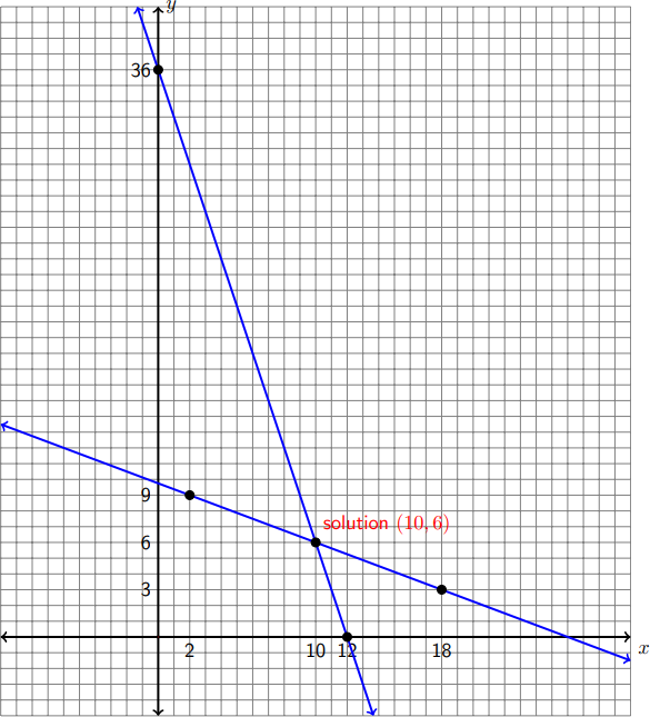
To solve this system by graphing, we start by graphing each of the given linear equations.

First, we graph $6 x+2 y=72$. Remember, we find two points:

\[x=0 \quad \Longrightarrow \quad y=36\nonumber\]

\[y=0 \quad \Longrightarrow \quad x=12\nonumber\]

Similarly, we graph $3 x+8 y=78$ by finding two points on this line:

\[x=2 \quad \Longrightarrow \quad y=9\nonumber\]

\[y=3 \quad \Longrightarrow \quad x=18\nonumber\]

The lines are graphed in the same coordinate system as shown below.

$imageedit_17_7405436324.png$

The coordinates of the point of intersection of the two graphs are the solution of the system. Observe from the graph that the $x$ and $y$ coordinates of the point of intersection are $x=10$ and $y=6$.

Example $\PageIndex{1}$

Solve by graphing:

\[\left(\begin{array}{lllll}
x & + & y & = & 7 \\
5 x & + & 10 y & = & 40
\end{array}\right)\nonumber\]

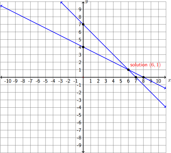
Step 1 Graph both lines:

\[\begin{align*}
x+y=7: \quad & x=0, y=7 \\
& y=0, x=7
\end{align*}\nonumber\]

\[\begin{align*}
5x + 10y = 40: \quad & x = 0, y = 4 \\
& y = 0, x = 8
\end{align*}\nonumber\]

$imageedit_20_6483886603.png$

Step 2 Read off the coordinates of the point of intersection:

\[x=6, y=1\nonumber\]

Step 3 The solution of the system is $x=6, y=1$.

Remark 28.3

If the graphs of the two lines do not have a point of intersection, then the system has no solution.
If the graphs of the lines coincide, then the system has infinitely many solutions.

Solving a System ot Two Linear Equations by Graphing

Step 1: Graph each linear equation on the same coordinate system.
Step 2: Label the point of intersection on the graph (if there is any).
Step 3: Read off the coordinates of the point of intersection (if possible). If the lines coincide, every point on them is considered an intersection point.
Step 4: Depending on Step 3, state whether the system has no solution (lines are parallel), infinitely many solutions (lines coincide), or one solution (single intersection point).

Exit Problem

Solve graphically:

$\begin{array}{lllll}
8 x & - & 4 y & = & 4 \\
3 x & - & 2 y & = & 3
\end{array}$