
8.4: Inverse Function
- Page ID
- 19730

\( \newcommand{\vecs}[1]{\overset { \scriptstyle \rightharpoonup} {\mathbf{#1}} } \)
\( \newcommand{\vecd}[1]{\overset{-\!-\!\rightharpoonup}{\vphantom{a}\smash {#1}}} \)
\( \newcommand{\dsum}{\displaystyle\sum\limits} \)
\( \newcommand{\dint}{\displaystyle\int\limits} \)
\( \newcommand{\dlim}{\displaystyle\lim\limits} \)
\( \newcommand{\id}{\mathrm{id}}\) \( \newcommand{\Span}{\mathrm{span}}\)
( \newcommand{\kernel}{\mathrm{null}\,}\) \( \newcommand{\range}{\mathrm{range}\,}\)
\( \newcommand{\RealPart}{\mathrm{Re}}\) \( \newcommand{\ImaginaryPart}{\mathrm{Im}}\)
\( \newcommand{\Argument}{\mathrm{Arg}}\) \( \newcommand{\norm}[1]{\| #1 \|}\)
\( \newcommand{\inner}[2]{\langle #1, #2 \rangle}\)
\( \newcommand{\Span}{\mathrm{span}}\)
\( \newcommand{\id}{\mathrm{id}}\)
\( \newcommand{\Span}{\mathrm{span}}\)
\( \newcommand{\kernel}{\mathrm{null}\,}\)
\( \newcommand{\range}{\mathrm{range}\,}\)
\( \newcommand{\RealPart}{\mathrm{Re}}\)
\( \newcommand{\ImaginaryPart}{\mathrm{Im}}\)
\( \newcommand{\Argument}{\mathrm{Arg}}\)
\( \newcommand{\norm}[1]{\| #1 \|}\)
\( \newcommand{\inner}[2]{\langle #1, #2 \rangle}\)
\( \newcommand{\Span}{\mathrm{span}}\) \( \newcommand{\AA}{\unicode[.8,0]{x212B}}\)
\( \newcommand{\vectorA}[1]{\vec{#1}} % arrow\)
\( \newcommand{\vectorAt}[1]{\vec{\text{#1}}} % arrow\)
\( \newcommand{\vectorB}[1]{\overset { \scriptstyle \rightharpoonup} {\mathbf{#1}} } \)
\( \newcommand{\vectorC}[1]{\textbf{#1}} \)
\( \newcommand{\vectorD}[1]{\overrightarrow{#1}} \)
\( \newcommand{\vectorDt}[1]{\overrightarrow{\text{#1}}} \)
\( \newcommand{\vectE}[1]{\overset{-\!-\!\rightharpoonup}{\vphantom{a}\smash{\mathbf {#1}}}} \)
\( \newcommand{\vecs}[1]{\overset { \scriptstyle \rightharpoonup} {\mathbf{#1}} } \)
\(\newcommand{\longvect}{\overrightarrow}\)
\( \newcommand{\vecd}[1]{\overset{-\!-\!\rightharpoonup}{\vphantom{a}\smash {#1}}} \)
\(\newcommand{\avec}{\mathbf a}\) \(\newcommand{\bvec}{\mathbf b}\) \(\newcommand{\cvec}{\mathbf c}\) \(\newcommand{\dvec}{\mathbf d}\) \(\newcommand{\dtil}{\widetilde{\mathbf d}}\) \(\newcommand{\evec}{\mathbf e}\) \(\newcommand{\fvec}{\mathbf f}\) \(\newcommand{\nvec}{\mathbf n}\) \(\newcommand{\pvec}{\mathbf p}\) \(\newcommand{\qvec}{\mathbf q}\) \(\newcommand{\svec}{\mathbf s}\) \(\newcommand{\tvec}{\mathbf t}\) \(\newcommand{\uvec}{\mathbf u}\) \(\newcommand{\vvec}{\mathbf v}\) \(\newcommand{\wvec}{\mathbf w}\) \(\newcommand{\xvec}{\mathbf x}\) \(\newcommand{\yvec}{\mathbf y}\) \(\newcommand{\zvec}{\mathbf z}\) \(\newcommand{\rvec}{\mathbf r}\) \(\newcommand{\mvec}{\mathbf m}\) \(\newcommand{\zerovec}{\mathbf 0}\) \(\newcommand{\onevec}{\mathbf 1}\) \(\newcommand{\real}{\mathbb R}\) \(\newcommand{\twovec}[2]{\left[\begin{array}{r}#1 \\ #2 \end{array}\right]}\) \(\newcommand{\ctwovec}[2]{\left[\begin{array}{c}#1 \\ #2 \end{array}\right]}\) \(\newcommand{\threevec}[3]{\left[\begin{array}{r}#1 \\ #2 \\ #3 \end{array}\right]}\) \(\newcommand{\cthreevec}[3]{\left[\begin{array}{c}#1 \\ #2 \\ #3 \end{array}\right]}\) \(\newcommand{\fourvec}[4]{\left[\begin{array}{r}#1 \\ #2 \\ #3 \\ #4 \end{array}\right]}\) \(\newcommand{\cfourvec}[4]{\left[\begin{array}{c}#1 \\ #2 \\ #3 \\ #4 \end{array}\right]}\) \(\newcommand{\fivevec}[5]{\left[\begin{array}{r}#1 \\ #2 \\ #3 \\ #4 \\ #5 \\ \end{array}\right]}\) \(\newcommand{\cfivevec}[5]{\left[\begin{array}{c}#1 \\ #2 \\ #3 \\ #4 \\ #5 \\ \end{array}\right]}\) \(\newcommand{\mattwo}[4]{\left[\begin{array}{rr}#1 \amp #2 \\ #3 \amp #4 \\ \end{array}\right]}\) \(\newcommand{\laspan}[1]{\text{Span}\{#1\}}\) \(\newcommand{\bcal}{\cal B}\) \(\newcommand{\ccal}{\cal C}\) \(\newcommand{\scal}{\cal S}\) \(\newcommand{\wcal}{\cal W}\) \(\newcommand{\ecal}{\cal E}\) \(\newcommand{\coords}[2]{\left\{#1\right\}_{#2}}\) \(\newcommand{\gray}[1]{\color{gray}{#1}}\) \(\newcommand{\lgray}[1]{\color{lightgray}{#1}}\) \(\newcommand{\rank}{\operatorname{rank}}\) \(\newcommand{\row}{\text{Row}}\) \(\newcommand{\col}{\text{Col}}\) \(\renewcommand{\row}{\text{Row}}\) \(\newcommand{\nul}{\text{Nul}}\) \(\newcommand{\var}{\text{Var}}\) \(\newcommand{\corr}{\text{corr}}\) \(\newcommand{\len}[1]{\left|#1\right|}\) \(\newcommand{\bbar}{\overline{\bvec}}\) \(\newcommand{\bhat}{\widehat{\bvec}}\) \(\newcommand{\bperp}{\bvec^\perp}\) \(\newcommand{\xhat}{\widehat{\xvec}}\) \(\newcommand{\vhat}{\widehat{\vvec}}\) \(\newcommand{\uhat}{\widehat{\uvec}}\) \(\newcommand{\what}{\widehat{\wvec}}\) \(\newcommand{\Sighat}{\widehat{\Sigma}}\) \(\newcommand{\lt}{<}\) \(\newcommand{\gt}{>}\) \(\newcommand{\amp}{&}\) \(\definecolor{fillinmathshade}{gray}{0.9}\)As we saw in the last section, in order to solve application problems involving exponential functions, we will need to be able to solve exponential equations such as
\(1500 = 1000e^{0.06t}\) or \(300 = 2^x\).
However, we currently don’t have any mathematical tools at our disposal to solve for a variable that appears as an exponent, as in these equations. In this section, we will develop the concept of an inverse function, which will in turn be used to define the tool that we need, the logarithm, in Section 8.5.
One-to-One Functions
A given function f is said to be one-to-one if for each value y in the range of f, there is just one value x in the domain of f such that y = f(x). In other words, f is one-to-one if each output y of f corresponds to precisely one input x.
It’s easiest to understand this definition by looking at mapping diagrams and graphs of some example functions.
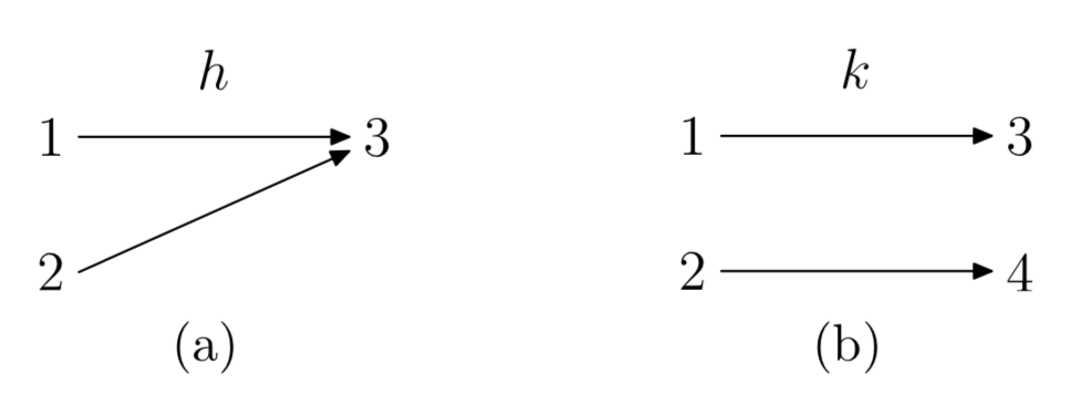
Consider the two functions h and k defined according to the mapping diagrams in Figure 1. In Figure 1(a), there are two values in the domain that are both mapped onto 3 in the range. Hence, the function h is not one-to-one. On the other hand, in Figure 1(b), for each output in the range of k, there is only one input in the domain that gets mapped onto it. Therefore, k is a one-to-one function.
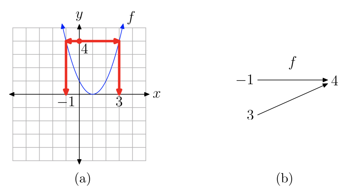
The graph of a function is shown in Figure 2(a). For this function f, the y-value 4 is the output corresponding to two input values, x = −1 and x = 3 (see the corresponding mapping diagram in Figure 2(b)). Therefore, f is not one-to-one.
Graphically, this is apparent by drawing horizontal segments from the point (0,4) on the y-axis over to the corresponding points on the graph, and then drawing vertical segments to the x-axis. These segments meet the x-axis at −1 and 3.
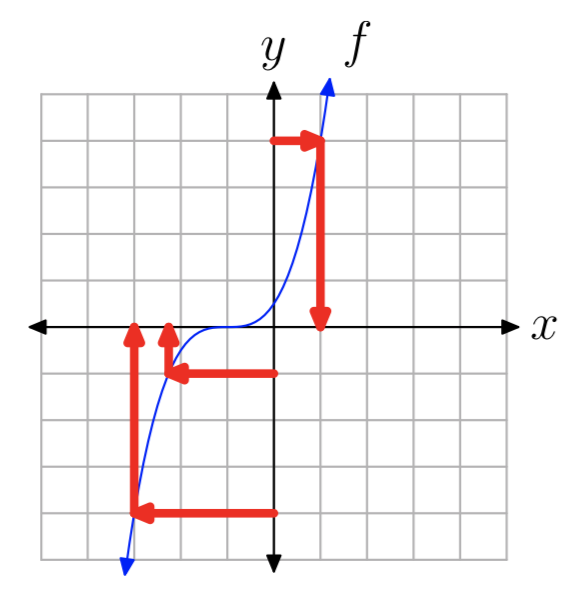
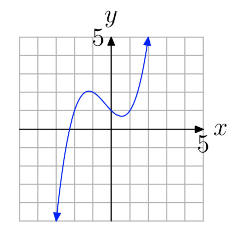
In Figure 3, each y-value in the range of f corresponds to just one input value x. Therefore, this function is one-to-one.
Graphically, this can be seen by mentally drawing a horizontal segment from each point on the y-axis over to the corresponding point on the graph, and then drawing a vertical segment to the x-axis. Several examples are shown in Figure 3. It’s apparent that this procedure will always result in just one corresponding point on the x-axis, because each y-value only corresponds to one point on the graph. In fact, it’s easiest to just note that since each horizontal line only intersects the graph once, then there can be only one corresponding input to each output.
The graphical process described in the previous example, known as the horizontal line test, provides a simple visual means of determining whether a function is one-to-one.
If each horizontal line intersects the graph of f at most once, then f is one-to-one. On the other hand, if some horizontal line intersects the graph of f more than once, then f is not one-to-one.
Remark 5. It follows from the horizontal line test that if f is a strictly increasing function, then f is one-to-one. Likewise, every strictly decreasing function is also one-to-one.
Inverse Functions
If f is one-to-one, then we can define an associated function g, called the inverse function of f. We will give a formal definition below, but the basic idea is that the inverse function g simply sends the outputs of f back to their corresponding inputs. In other words, the mapping diagram for g is obtained by reversing the arrows in the mapping diagram for f.
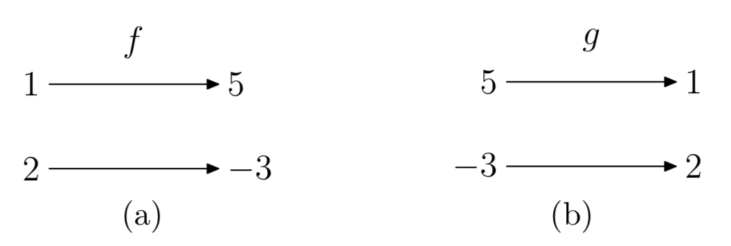
The function f in Figure 4(a) maps 1 to 5 and 2 to −3. Therefore, the inverse function g in Figure 4(b) maps the outputs of f back to their corresponding inputs: 5 to 1 and −3 to 2. Note that reversing the arrows on the mapping diagram for f yields the mapping diagram for g.
Since the inverse function g sends the outputs of f back to their corresponding inputs, it follows that the inputs of g are the outputs of f, and vice versa. Thus, the functions g and f are related by simply interchanging their inputs and outputs.
The original function must be one-to-one in order to have an inverse. For example, consider the function h in Example 2. h is not one-to-one. If we reverse the arrows in the mapping diagram for h (see Figure 1(a)), then the resulting relation will not be a function, because 3 would map to both 1 and 2.
Before giving the formal definition of an inverse function, it’s helpful to review the description of a function given in Section 2.1. While functions are often defined by means of a formula, remember that in general a function is just a rule that dictates how to associate a unique output value to each input value.
Suppose that f is a given one-to-one function. The inverse function g is defined as follows: for each y in the range of f, define g(y) to be the unique value x such that y = f(x).
To understand this definition, it’s helpful to look at a diagram:
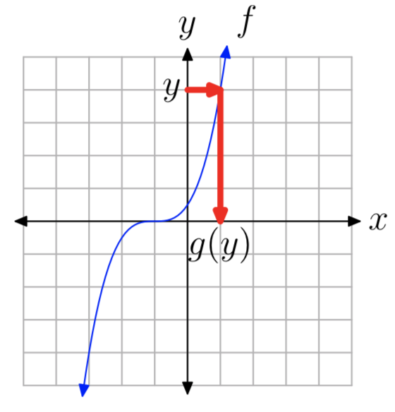
The input for g is any y-value in the range of f. Thus, the input in the above diagram is a value on the y-axis. The output of g is the corresponding value on the x-axis which satisfies the condition y = f(x). Note in particular that the x-value is unique because f is one-to-one.
The relationship between the original function f and its inverse function g can be described by:
If g is the inverse function of f, then
\(x = g(y) \longleftrightarrow y = f(x)\).
In fact, this is really the defining relationship for the inverse function. An easy way to understand this relationship (and the entire concept of an inverse function) is to realize that it states that inputs and outputs are interchanged. The inputs of g are the outputs of f, and vice versa. It follows that the Domain and Range of f and g are interchanged:
If g is the inverse function of f, then
Domain(g) = Range(f) and Range(g) = Domain(f).
The defining relationship in Property 8 is also equivalent to the following two identities, so these provide an alternative characterization of inverse functions:
If g is the inverse function of f, then
g(f(x)) = x for every x in Domain(f)
and
f(g(y)) = y for every y in Domain(g).
Note that the first statement in Property 10 says that g maps the output f(x) back to the input x. The second statement says the same with the roles of f and g reversed. Therefore, f and g must be inverses.
Property 10 can also be interpreted to say that the functions g and f “undo” each other. If we first apply f to an input x, and then apply g, we get x back again. Likewise, if we apply g to an input y, and then apply f, we get y back again. So whatever action f performs, g reverses it, and vice versa.
Suppose \(f(x) = x^3\). Thus, f is the “cubing” function. What operation will reverse the cubing process? Taking a cube root. Thus, the inverse of f should be the function \(g(y) = \sqrt[3]{y}\).
Let’s verify Property 10:
\(g(f(x))=g(x^3)= \sqrt[3]{x^3} = x\)
and
\(f(g(y)) = f(\sqrt[3]{y}) = (\sqrt[3]{y})^3 = y\)
Suppose f(x) = 4x−1. f acts on an input x by first multiplying by 4, and then subtracting 1. The inverse function must reverse the process: first add 1, and then divide by 4. Thus, the inverse function should be \(g(y) = \frac{y+1}{4}\).
Again, let’s verify Property 10:
\(g(f(x)) = g(4x−1) = \frac{(4x−1)+1}{4} = \frac{4x}{4} = x\)
and
\(f(g(y)) = f(\frac{y+1}{4}) = 4(\frac{y+1}{4})−1 = (y+1)−1 = y\)
Remarks 13.
- The computation g(f(x)), in which the output of one function is used as the input of another, is called the composition of g with f. Thus, inverse functions “undo” each other in the sense of composition. Composition of functions is an important concept in many areas of mathematics, so more practice with composition of functions is provided in the exercises.
- If g is the inverse function of f, then f is also the inverse of g. This follows from either Property 8 or Property 10. (Note that the labels x and y for the variables are unimportant. The key idea is that two functions are inverses if their inputs and outputs are interchanged.)
Notation: In order to indicate that two functions f and g are inverses, we usually use the notation \(f^{−1}\) for g. The symbol \(f^{−1}\) is read “f inverse”. In addition, to avoid confusion with the typical roles of x and y, it’s often useful to use different labels for the variables. Rewriting Property 8 with the \(f^{−1}\) notation, and using new labels for the variables, we have the defining relationship:
\(v = f^{−1}(u) \longleftrightarrow u = f(v)\)
Likewise, rewriting Property 10, we have the composition relationships:
\(f^{−1}(f(z))\) = z for every z in Domain(f)
and
\(f(f^{−1}(z)) = z\) for every z in Domain(\(f^{−1}\))
However, the new notation comes with an important warning:
\(f^{−1}\) does not mean \(\frac{1}{f}\)
The −1 exponent is just notation in this context. When applied to a function, it stands for the inverse of the function, not the reciprocal of the function.
The Graph of an Inverse Function
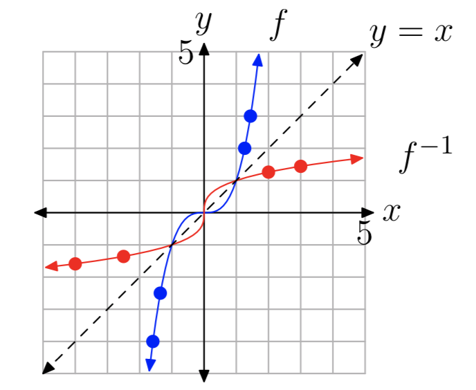
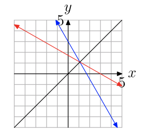
How are the graphs of f and \(f^{−1}\) related? Suppose that the point (a, b) is on the graph of f. That means that b = f(a). Since inputs and outputs are interchanged for the inverse function, it follows that \(a = f^{−1}(b)\), so (b, a) is on the graph of \(f^{−1}\). Now (a, b) and (b, a) are just reflections of each other across the line y = x (see the discussion below for a detailed explanation), so it follows that the same is true of the graphs of f and \(f^{−1}\) if we graph both functions on the same coordinate system (i.e., as functions of x).
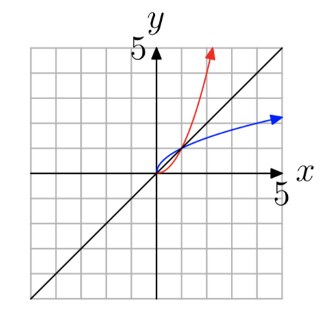
For example, consider the functions from Example 11. The functions \(f(x) = x^3\) and \(f^{−1}(x) = \sqrt[3]{x}\) are graphed in Figure 6 along with the line y = x. Several reflected pairs of points are also shown on the graph.
To see why the points (a, b) and (b, a) are just reflections of each other across the line y = x, consider the segment S between these two points (see Figure 7). It will be enough to show: (1) that S is perpendicular to the line y = x, and (2) that the intersection point P of the segment S and the line y = x is equidistant from each of(a, b) and (b, a).
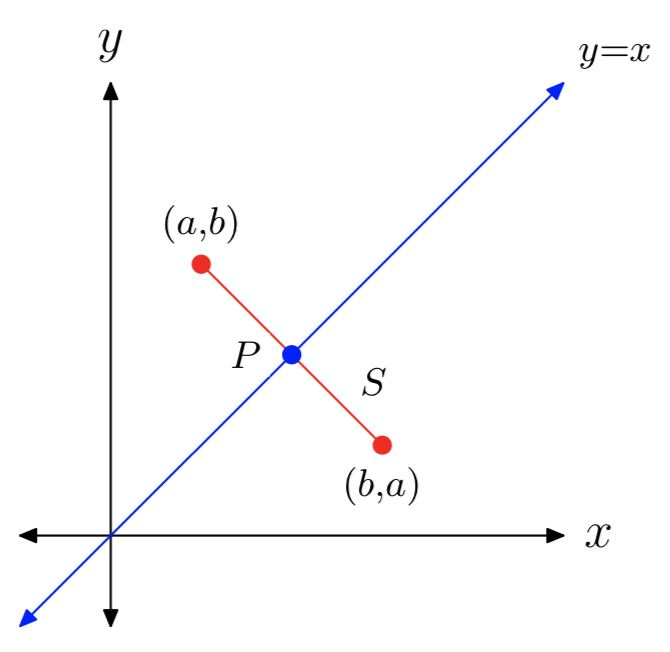
- The slope of S is
\(\frac{a−b}{b−a} = −1\),
and the slope of the line y = x is 1, so they are perpendicular.
2. The line containing S has equation y−b = −(x−a), or equivalently, y = −x+(a+b). To find the intersection of S and the line y = x, set x = −x+(a+b) and solve for x to get
\(x = \frac{a+b}{2}\).
Since y = x, it follows that the intersection point is
\(P = (\frac{a+b}{2}, \frac{a+b}{2})\)
Finally, we can use the distance formula presented in section 9.6 to compute the distance from P to (a, b) and the distance from P to (b, a). In both cases, the computed distance turns out to be
\(\frac{|a−b|}{\sqrt{2}}\)
Computing the Formula of an Inverse Function
How does one find the formula of an inverse function? In Example 11, it was easy to see that the inverse of the “cubing” function must be the cube root function. But how was the formula for the inverse in Example 12 obtained?
Actually, there is a simple procedure for finding the formula for the inverse function (provided that such a formula exists; remember that not all functions can be described by a simple formula, so the procedure will not work for such functions). The following procedure works because the inputs and outputs (the x and y variables) are switched in step 3.
- Check the graph of the original function f(x) to see if it passes the horizontal line test. If so, then f is one-to-one and you can proceed.
- Write the formula in xy-equation form, as y = f(x).
- Interchange the x and y variables.
- Solve the new equation for y, if possible. The result will be the formula for \(f^{−1}(x)\).
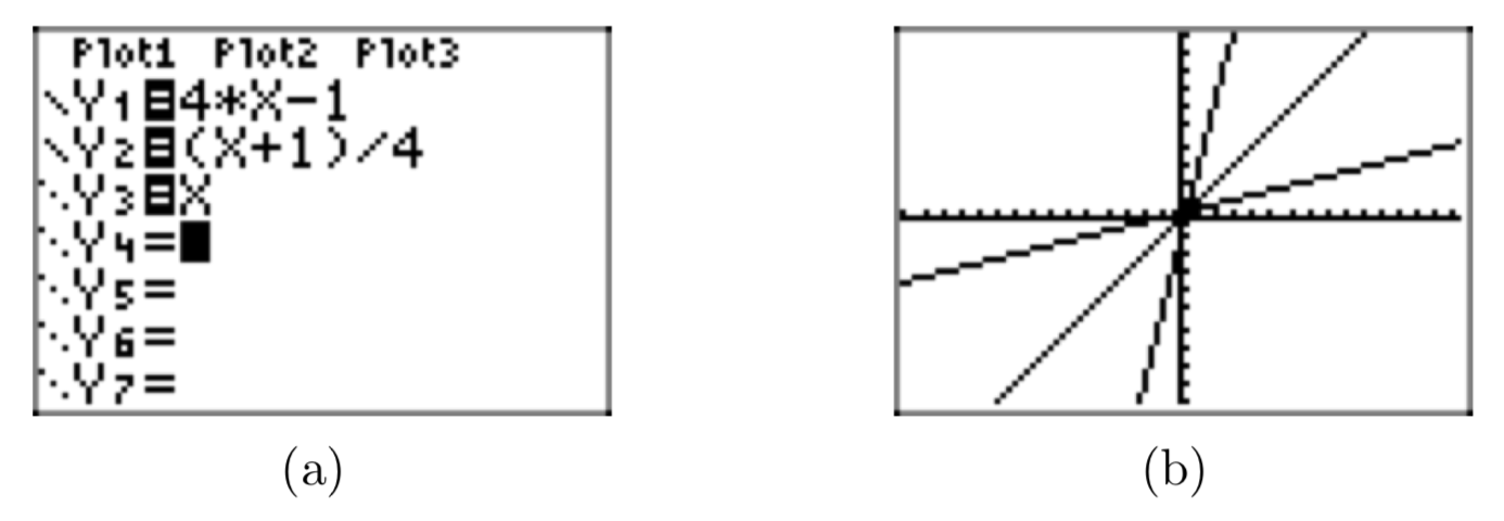
Let’s start by finding the inverse of the function f(x) = 4x−1 from Example 12.
Step 1: A check of the graph shows that f is one-to-one (see Figure 8).
STEP 2: Write the formula in xy-equation form: y = 4x − 1
STEP 3: Interchange x and y: x = 4y − 1
STEP 4: Solve for y:
x = 4y − 1
\(\rightarrow x+1=4y\)
\(\rightarrow \frac{x+1}{4} = y\)
Thus, \(f^{−1}(x) = \frac{x+1}{4}\).
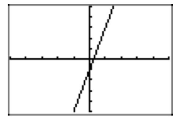
Figure 9 demonstrates that the graph of \(f^{−1}(x) = \frac{x+1}{4}\) is a reflection of the graph of f (x) = 4x−1 across the line y = x. In this figure, the ZSquare command in the ZOOM menu has been used to better illustrate the reflection (the ZSquare command equalizes the scales on both axes).
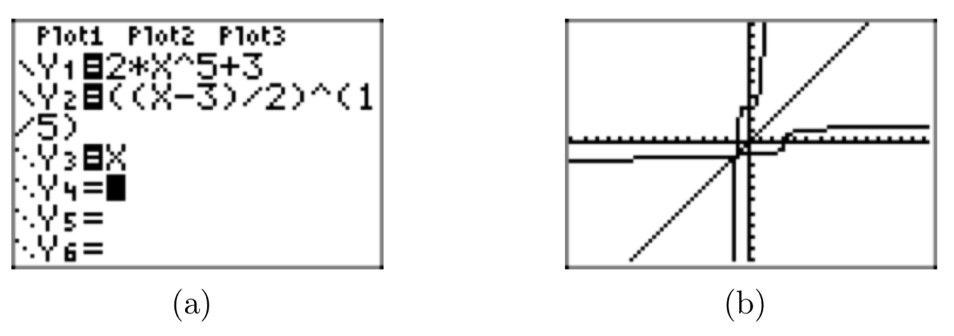
This time we’ll find the inverse of \(f(x) = 2x^5+3\).
Step 1: A check of the graph shows that f is one-to-one (this is left for the reader to verify).
STEP 2: Write the formula in xy-equation form: \(y = 2x^5+3\).
STEP 3: Interchange x and y: \(x = 2y^5+3\).
STEP 4: Solve for y:
\(x = 2y^5+3\).
\(\rightarrow x−3 = 2y^5\)
\(\rightarrow \frac{x−3}{2} = y^5\)
\(\rightarrow \sqrt[5]{\frac{x−3}{2}} = y\)
Thus, \(f^{−1}(x) = \sqrt[5]{\frac{x−3}{2}}\)
Again, note that the graph of \(f^{−1}(x) = \sqrt[5]{\frac{x−3}{2}}\) is a reflection of the graph of \(f(x) = 2x^5+3\) across the line y = x (see Figure 10).
Find the inverse of \(f(x) = \frac{5}{7+x}\).
Step 1: A check of the graph shows that f is one-to-one (this is left for the reader to verify).
STEP 2: Write the formula in xy-equation form: \(y = \frac{5}{7+x}\).
STEP 3: Interchange x and y: \(x = \frac{5}{7+y}\).
STEP 4: Solve for y:
\(x = \frac{5}{7+y}\)
\(\rightarrow x(7+y) = 5\)
\(\rightarrow 7+y = \frac{5}{x}\)
\(y = \frac{5}{x}−7 = \frac{5 − 7x}{x}\)
Thus, \(f^{−1}(x) = \frac{5 − 7x}{x}\)
This example is a bit more complicated: find the inverse of the function \(f(x) = \frac{5x+2}{x−3}\).
Step 1: A check of the graph shows that f is one-to-one (this is left for the reader to verify).
STEP 2: Write the formula in xy-equation form: \(y = \frac{5x+2}{x−3}\).
STEP 3: Interchange x and y: \(x = \frac{5y+2}{y−3}\).
STEP 4: Solve for y:
\(x = \frac{5y+2}{y−3}\)
\(\rightarrow x(y−3) = 5y+2\)
\(\rightarrow xy−3x = 5y+2\)
This equation is linear in y. Isolate the terms containing the variable y on one side of the equation, factor, then divide by the coefficient of y.
\(xy−3x = 5y+2\)
\(xy−5y = 3x+2\)
\(y(x−5) = 3x+2\)
\(y = \frac{3x+2}{x−5}\)
Thus, \(f^{−1}(x) = \frac{3x+2}{x−5}\).
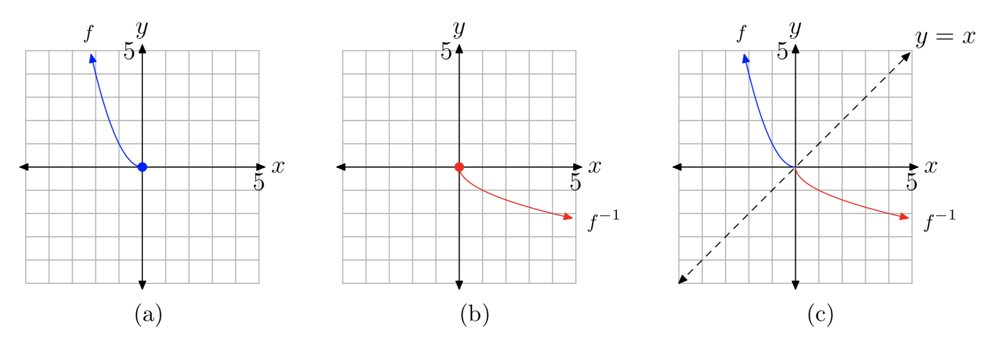
According to the horizontal line test, the function \(h(x) = x^2\) is certainly not one-to-one. However, if we only consider the right half or left half of the function (i.e., restrict the domain to either the interval \([0, \infty)\) or \((−\infty,0]\)), then the function would be one-to-one, and therefore would have an inverse (Figure 11(a) shows the left half). For example, suppose f is the function \(f(x) = x^2\), \(x \le 0\)
In this case, the procedure still works, provided that we carry along the domain condition in all of the steps, as follows:
Step 1: The graph in Figure 11(a) passes the horizontal line test, so f is one-to-one.
Step 2: Write the formula in xy-equation form: \(y = x^2\), \(x \le 0\)
Step 3: Interchange x and y: \(x = y^2\), \(y \le 0\)
Note how x and y must also be interchanged in the domain condition.
Step 4: Solve for y: \(y = \pm \sqrt{x}\), \(y \le 0\)
Now there are two choices for y, one positive and one negative, but the condition \(y \le 0\) tells us that the negative choice is the correct one. Thus, the last statement is equivalent to
\(y = −\sqrt{x}\).
Thus, \(f^{−1}(x) = −\sqrt{x}\). The graph of \(f^{−1}\) is shown in Figure 11(b), and the graphs of both f and \(f^{−1}\) are shown in Figure 11(c) as reflections across the line y = x.
Exercise
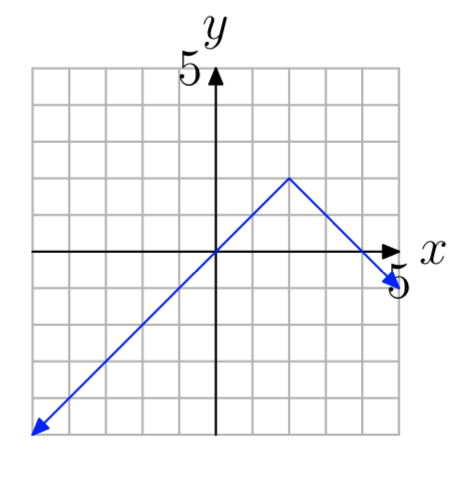
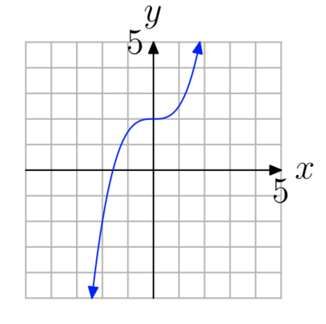
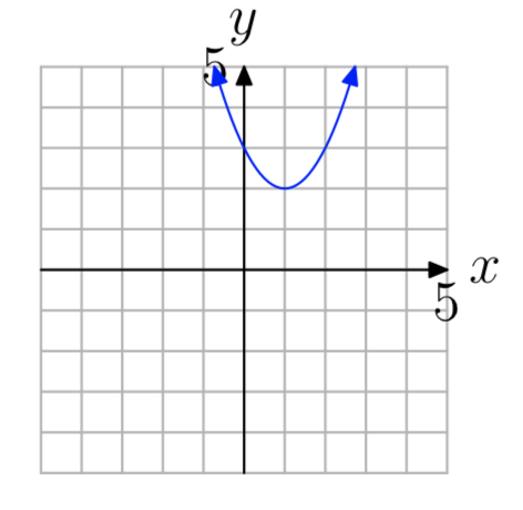
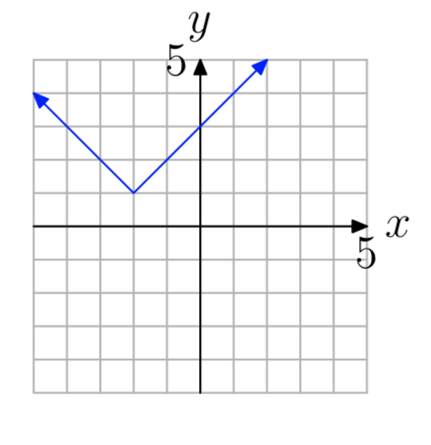
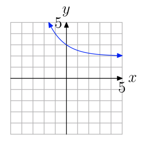
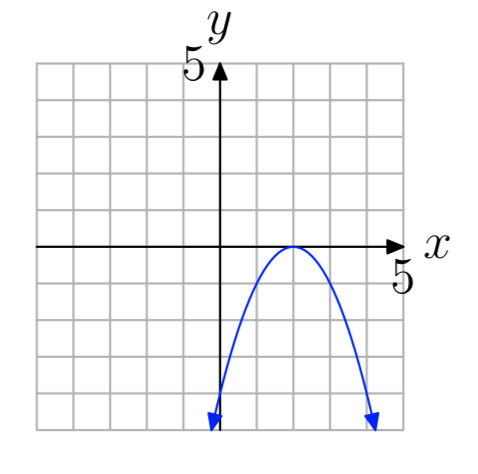
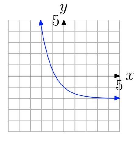
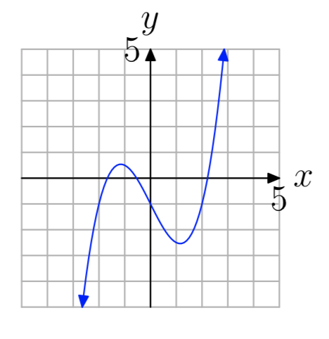
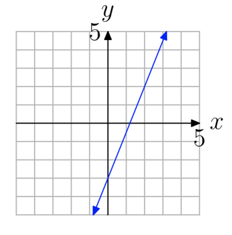
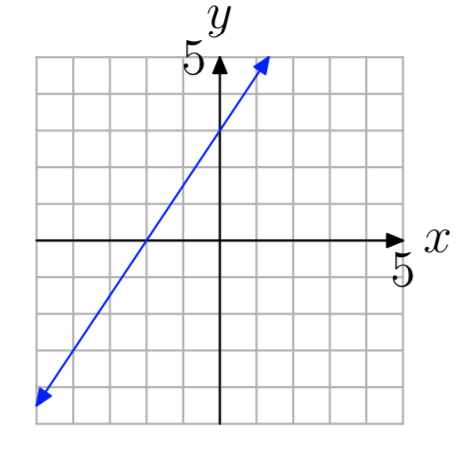
In Exercises 1-12, use the graph to determine whether the function is one-to-one.
- Answer
-
not one-to-one

- Answer
-
not one-to-one
- Answer
-
not one-to-one
- Answer
-
one-to-one
- Answer
-
one-to-one
- Answer
-
one-to-one
In Exercises 13-28, evaluate the composition g(f(x)) and simplify your answer.
\(g(x) = \frac{9}{x}\), \(f(x) = −2x^2+5x−2\)
- Answer
-
\(\frac{−9}{2x^2−5x+2}\)
\(f(x) = −\frac{5}{x}\), \(g(x) = −4x^2+x−1\)
\(g(x) = 2\sqrt{x}\), \(f(x)=−x−3\)
- Answer
-
\(2\sqrt{−x−3}\)
\(f(x) = 3x^2−3x−5\), \(g(x) = \frac{6}{x}\)
\(g(x) = 3\sqrt{x}\), \(f(x) = 4x+1\)
- Answer
-
\(3\sqrt{4x+1}\)
f(x) = −3x−5, g(x)=−x−2
\(g(x) = −5x^2+3x−4\), \(f(x) = \frac{5}{x}\)
- Answer
-
\(−\frac{125}{x^2}+\frac{15}{x}−4\)
g(x) = 3x+3, \(f(x) = 4x^2 −2x−2\)
\(g(x) = 6\sqrt{x}\), f(x) = −4x+4
- Answer
-
\(6\sqrt{−4x+4}\)
g(x) = 5x−3, f(x)=−2x−4
\(g(x) = 3\sqrt{x}\), f(x) = −2x+1
- Answer
-
\(3\sqrt{−2x+1}\)
\(g(x) = \frac{3}{x}\), \(f(x)=−5x^2−5x−4\)
\(f(x)=\frac{5}{x}\), g(x)=−x+1
- Answer
-
\(−\frac{5}{x}+1\)
\(f(x) = 4x^2+3x−4\), \(g(x) = \frac{2}{x}\)
g(x) = −5x+1, f(x) = −3x−2
- Answer
-
15x+11
\(g(x) = 3x^2 +4x−3\), \(f(x)=\frac{8}{x}\)
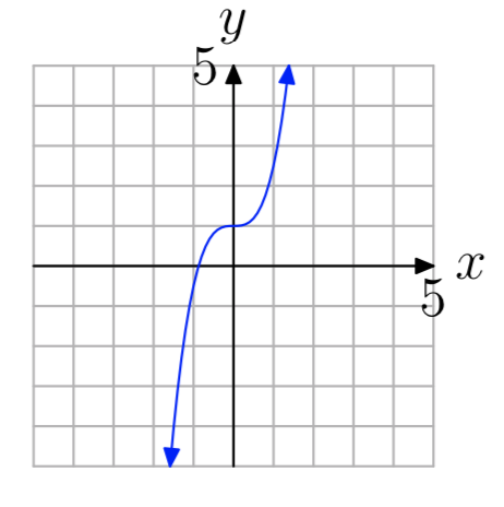
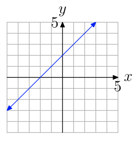
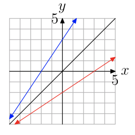
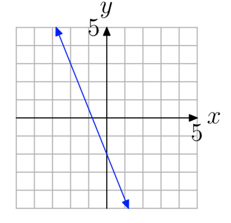
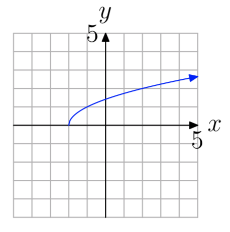
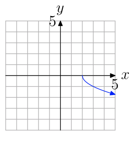
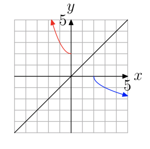
In Exercises 29-36, first copy the given graph of the one-to-one function f(x) onto your graph paper. Then on the same coordinate system, sketch the graph of the inverse function \(f^{−1}(x)\).
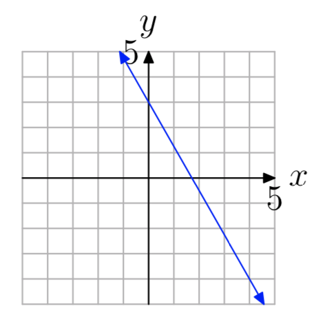
- Answer
-
- Answer
-

- Answer
-
- Answer
-
In Exercises 37-68, find the formula for the inverse function \(f^{−1}(x)\).
\(f(x) = 5x^3−5\)
- Answer
-
\(\sqrt[3]{\frac{x+5}{5}}\)
\(f(x) = 4x^7−3\)
\(f(x)=−\frac{9x−3}{7x+6}\)
- Answer
-
\(−\frac{6x−3}{7x+9}\)
f(x) = 6x−4
f(x) = 7x−9
- Answer
-
\(\frac{x+9}{7}\)
f(x) = 7x+4
\(f(x) = 3x^5−9\)
- Answer
-
\(\sqrt[5]{\frac{x+9}{3}}\)
f(x) = 6x+7
\(f(x) = \frac{4x+2}{4x+3}\)
- Answer
-
\(−\frac{3x−2}{4x−4}\)
\(f(x) = 5x^7+4\)
\(f(x) = \frac{4x−1}{2x+2}\)
- Answer
-
\(−\frac{2x+1}{2x−4}\)
\(f(x) = \sqrt[7]{8x−3}\)
\(f(x) = \sqrt[3]{−6x−4}\)
- Answer
-
\(−\frac{x^3+4}{6}\)
\(f(x) = \frac{8x−7}{3x−6}\)
\(f(x) = \sqrt[7]{−3x−5}\)
- Answer
-
\(−\frac{x^7+5}{3}\)
\(f(x) = \sqrt[9]{8x+2}\)
\(f(x) = \sqrt[3]{6x+7}\)
- Answer
-
\(\frac{x^3−7}{6}\)
\(f(x) = \frac{3x+7}{2x+8}\)
f(x) = −5x+2
- Answer
-
\(−\frac{x−2}{5}\)
f(x) = 6x+8
\(f(x) = 9x^9+5\)
- Answer
-
\(\sqrt[9]{\frac{x−5}{9}}\)
\(f(x) = 4x^5−9\)
\(f(x) = \frac{9x−3}{9x+7}\)
- Answer
-
\(−\frac{7x+3}{9x−9}\)
\(f(x) = \sqrt[3]{9x−7}\)
\(f(x) = x^4\), \(x \le 0\)
- Answer
-
\(−\sqrt[4]{x}\)
\(f(x) = x^4\), \(x \ge 0\)
\(f(x) = x^2−1\), \(x \le 0\)
- Answer
-
\(−\sqrt{x+1}\)
\(f(x) = x^2+2\), \(x \ge 0\)
\(f(x) = x^4+3\), \(x \le 0\)
- Answer
-
\(−\sqrt[4]{x−3}\)
\(f(x) = x^4−5\), \(x \ge 0\)
\(f(x) = (x−1)^2\), \(x \le 1\)
- Answer
-
\(−\sqrt{x}+1\)
\(f(x) = (x+2)^2\), \(x \ge −2\)