8.5: Logarithmic Functions

We can now apply the inverse function theory from the previous section to the exponential function. From Section 8.2, we know that the function $f(x) = b^x$ is either increasing (if b > 1) or decreasing (if 0 < b < 1), and therefore is one-to-one. Consequently, f has an inverse function $f^{−1}$.

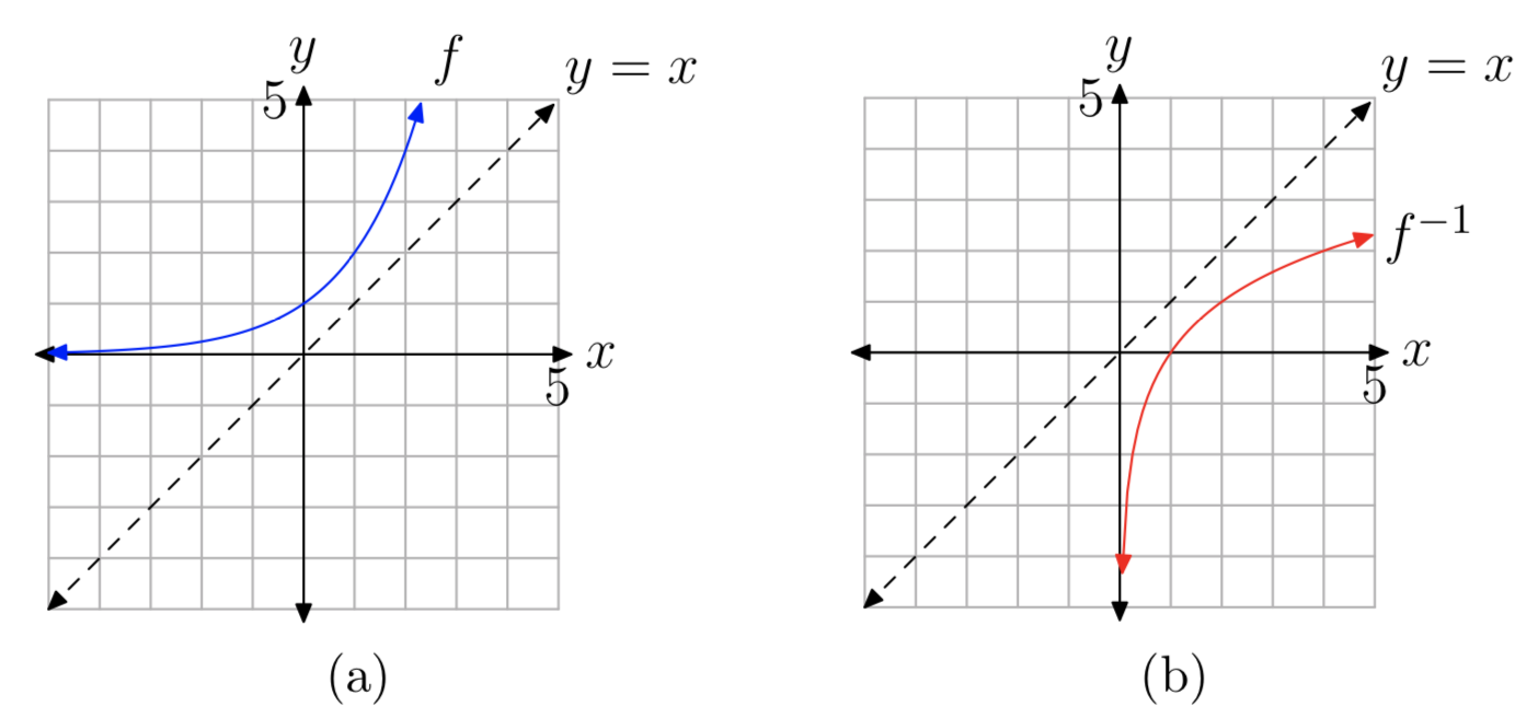
As an example, let’s consider the exponential function $f(x) = 2^x$. f is increasing, has domain $D_{f} = (−\infty, \infty)$, and range $R_{f} = (0, \infty)$. Its graph is shown in Figure 1(a). The graph of the inverse function $f^{−1}$ is a reflection of the graph of f across the line y = x, and is shown in Figure 1(b). Since domains and ranges are interchanged, the domain of the inverse function is $D_{f^{−1}} = (0, \infty)$ and the range is $R_{f^{−1}} = (−\infty, \infty)$.

Figure 1. The graphs of $f(x) = 2^x$ and its inverse $f^{−1}(x)$ are reflections across the line y = x.

Unfortunately, when we try to use the procedure given in Section 8.4 to find a formula for $f^{−1}$, we run into a problem. Starting with $y = 2^x$, we then interchange x and y to obtain $x = 2^y$. But now we have no algebraic method for solving this last equation for y. It follows that the inverse of $f(x) = 2^x$ has no formula involving the usual arithmetic operations and functions that we’re familiar with. Thus, the inverse function is a new function. The name of this new function is the logarithm of x to base 2, and it’s denoted by $f^{−1}(x) = log_{2}(x)$.

Recall that the defining relationship between a function and its inverse (Property 14 in Section 8.4) simply states that the inputs and outputs of the two functions are interchanged. Thus, the relationship between $2^x$ and its inverse $log_{2}(x)$ takes the following form:

$v = log_{2}(u) \longleftrightarrow u = 2^v$

More generally, for each exponential function $f(x) = b^x$ (b > 0, $b \ne 1$), the inverse function $f^{−1}(x)$ is called the logarithm of x to base b, and is denoted by $log_{b}(x)$. The defining relationship is given in the following definition.

Definition $\PageIndex{1}$

If b > 0 and $b \ne 1$, then the logarithm of u to base b is defined by the relationship

$v = log_{b}(u) \longleftrightarrow u = b^v$. (2)

In order to understand the logarithm function better, let’s work through a few simple examples.

Example $\PageIndex{3}$

Compute $log_{2}(8)$.

Answer

Label the required value by v, so $v = log_{2}(8)$. Then by (2), using b = 2 and u = 8, it follows that $2^v = 8$, and therefore v = 3 (solving by inspection).

In the last example, note that $log_{2}(8) = 3$ is the exponent v such that $2^v = 8$. Thus, in general, one way to interpret the definition of the logarithm in (2) is that $log_{b}(u)$ is the exponent v such that $b^v = u$. In other words, the value of the logarithm is the exponent!

Example $\PageIndex{4}$

Compute $log_{10}(10000)$.

Answer

Again, label the required value by v, so $v = log_{10}(10000)$. By (2), it follows that $10^v = 10 000$, and therefore v = 4. Note that here again we have found the exponent v = 4 that is needed for base 10 in order to get $10^v = 10 000$.

Example $\PageIndex{5}$

Compute $log_{3}(\frac{1}{9})$.

Answer

$v = log_{3}(\frac{1}{9})$

$\rightarrow 3^v = \frac{1}{9}$ by (2)

$\rightarrow v = −2$ since $3^{−2} = \frac{1}{9}$

Example $\PageIndex{6}$

Solve the equation $log_{5}(x) = 1$.

Answer

$log_{5}(x) = 1$

$\rightarrow 5^1 = x$ by (2)

$\rightarrow x = 5$

Example $\PageIndex{7}$

Solve the equation $log_{b}(64) = 3$ for b.

Answer

$log_{b}(64) = 3$

$\rightarrow b^3 = 64$ by (2)

$\rightarrow b = \sqrt[3]{64} = 4$

Example $\PageIndex{8}$

Solve the equation $log_{\frac{1}{2}}(x) = −2$.

Answer

$log_{\frac{1}{2}}(x) = −2$

$\rightarrow (\frac{1}{2})^{−2} = x$ by (2)

$\rightarrow \frac{1}{(\frac{1}{2})^2} = \frac{1}{\frac{1}{4}} = 4$

The composition relationships in Property 15 of Section 8.4, applied to $b^x$ and $log_{b}(x)$, become

PROPERTY $\PageIndex{9}$

$$log_{b}(b^x) = x \label{10}$$

and

$$b^{log_{b}(x)} = x \label{11}.$$

Both equations are important. Note that Equation $\ref{11}$ again shows that the $log_{b}(x)$ is the exponent v such that $b^v = x$. Equation $\ref{10}$ will be used frequently in this and later sections to help us solve exponential equations.

Logarithmic functions are used in many areas of science and engineering. For example, they are used to define the Richter scale for the magnitudes of earthquakes, the decibel scale for the loudness of sound, and the astronomical scale for stellar brightness. They are also important tools for use in computation (as we will see in Section 8.8). Our main use of logarithms in this textbook will be to solve exponential equations, and thereby help us study physical phenomena that are described by exponential functions (as in Section 8.7).

Computing Logarithms

In Examples 3–8 above, we were able to compute the logarithms by converting to exponential equations that could be solved by inspection. But it’s easy to see that most of the time this won’t work. For example, how would we compute the value of $log_{2}(7)$?

Fortunately, mathematicians have found other methods for computing logarithms to high accuracy, and they can now be easily approximated using a calculator or computer.

Your calculator has built-in buttons for computing two different logarithms, $log_{10}(x)$ and $log_{e}(x)$. $log_{10}(x)$ is called the common logarithm, and $log_{e}(x)$ is called the natural logarithm.

Common Logarithm: The common logarithm $log_{10}(x)$ is computed using the LOGbutton on your calculator. Notice also that its inverse function $10^x$, can be computed using the same button in conjunction with the 2ND button. The common logarithm is usually the most convenient one to use for computations involving scientific notation (because we use a base 10 number system), and therefore is the logarithm most often used in the physical sciences. Because of that, it’s often just abbreviated by log(x), and we’ll do that as well in the remainder of the text.

COMMON LOGARITHM

log(x) and $log_{10}(x)$ are equivalent notations. Thus, we have the defining relationship

$v = log(u) \longleftrightarrow u = 10^v$.

The composition properties for the common logarithm are

$log(10^x) = x$ (12)

and

$10^{log(x)} = x$.

Natural Logarithm: The natural logarithm \(log_{e}(x)\) is computed using the LNbutton on your calculator. Its inverse function, $e^x$, is computed using the same button in conjunction with the 2ND button. The natural logarithm turns out to be the most convenient one to use in mathematics, because a lot of formulas, especially in calculus, are much simpler when the natural logarithm is used. The natural logarithm is abbreviated by ln(x).

NATURAL LOGARITHM

ln(x) and $log_{e}(x)$ are equivalent notations. Thus, we have the defining relationship

$v = ln(u) \longleftrightarrow u = e^v$.

The composition properties for the common logarithm are

$$ln(e^x) = x \label{13}$$

and

$$e^{\ln(x)} = x \lable{14} \nonumber$$

Note that when using your calculator to compute log(x) and ln(x), you will usually only obtain approximate values, as these values frequently are irrational numbers.

What about other bases? You can also compute these on your calculator, but we’ll first need to develop the Change of Base Formula in the next section. However, at this point, we can at least solve exponential equations involving bases 10 and e, as shown in the next two examples.

Example $\PageIndex{14}$

Solve the equation $704 = 2(10)^{x}$.

Answer

The first step is to isolate the exponential on the right side by dividing both sides by 2:

$352 = 10^x$

Then simply apply the $log_{10}(x)$ function to both sides of the equation:

$log_{10}(352) = log_{10}(10^x)$

But (10) implies that $log_{10}(10^x) = x$. Therefore, $x = log_{10}(352) = log(352)$ is the exact solution. The approximate value, using a calculator, is 2.546542663 (see Figure 2). Alternatively, instead of taking the logarithm of both sides in the second step, you can apply (2) to the equation $352 = 10^x$ to get $x = log_{10}(352)$.

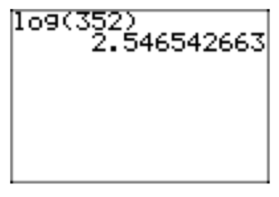
Figure 2. Approximation of $log(352) = log_{10}(352)$.

This last example shows how logarithms can be used for solving exponential equations. The basic strategy is to first isolate the exponential on one side of the equation, and then take appropriate logarithms of both sides. Here’s one more example for now, and then we’ll return to this process repeatedly in the remaining sections, especially when we work with application problems.

Example $\PageIndex{15}$

Solve the equation $30 = 20e^x$.

Answer

First isolate the exponential on the right side by dividing both sides by 20:

$1.5 = e^x$

This time, since the base of the exponential function is e, apply the natural logarithm function to both sides:

$log_{e}(1.5) = log_{e}(e^x)$

Simplify the right side, since $log_{e}(e^x) = x$ by (10):

$log_{e}(1.5) = x$

Therefore, $x = log_{e}(1.5) = ln(1.5)$ is the exact solution. The approximate value, using a calculator, is 0.4054651081 (see Figure 3).

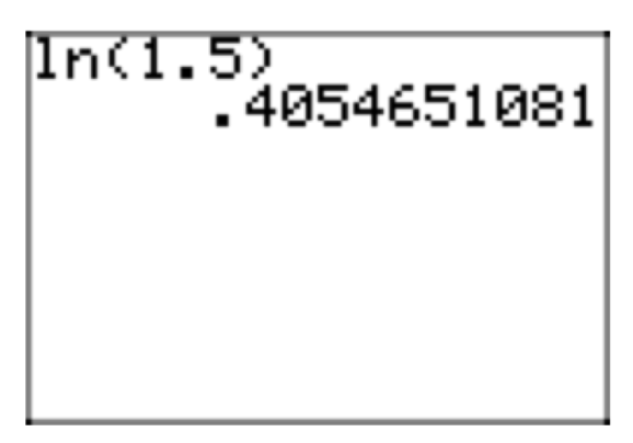
Figure 3. Approximation of $ln1.5 = log_{e}(1.5)$.

In the next section, we’ll learn how to solve exponential equations involving other bases.

Graphs of Logarithmic Functions

At the beginning of this section, we looked at the graphs of $f(x) = 2^x$ and its inverse function $f^{−1}(x) = log_{2}(x)$. More generally, the graph of the exponential function $f(x) = b^x$ for b > 1 is shown in Figure 4(a), along with its inverse logarithmic function $f^{−1}(x) = log_{b}(x)$. According to Section 8.4, the two graphs are reflections across the line y = x. Similarly, the graph for 0 < b < 1 is shown in Figure 4(b).

Figure 4. The graphs of $f(x) = b^x$ and $f^{−1}(x) = log_{b}(x)$ are reflections across the line y = x.

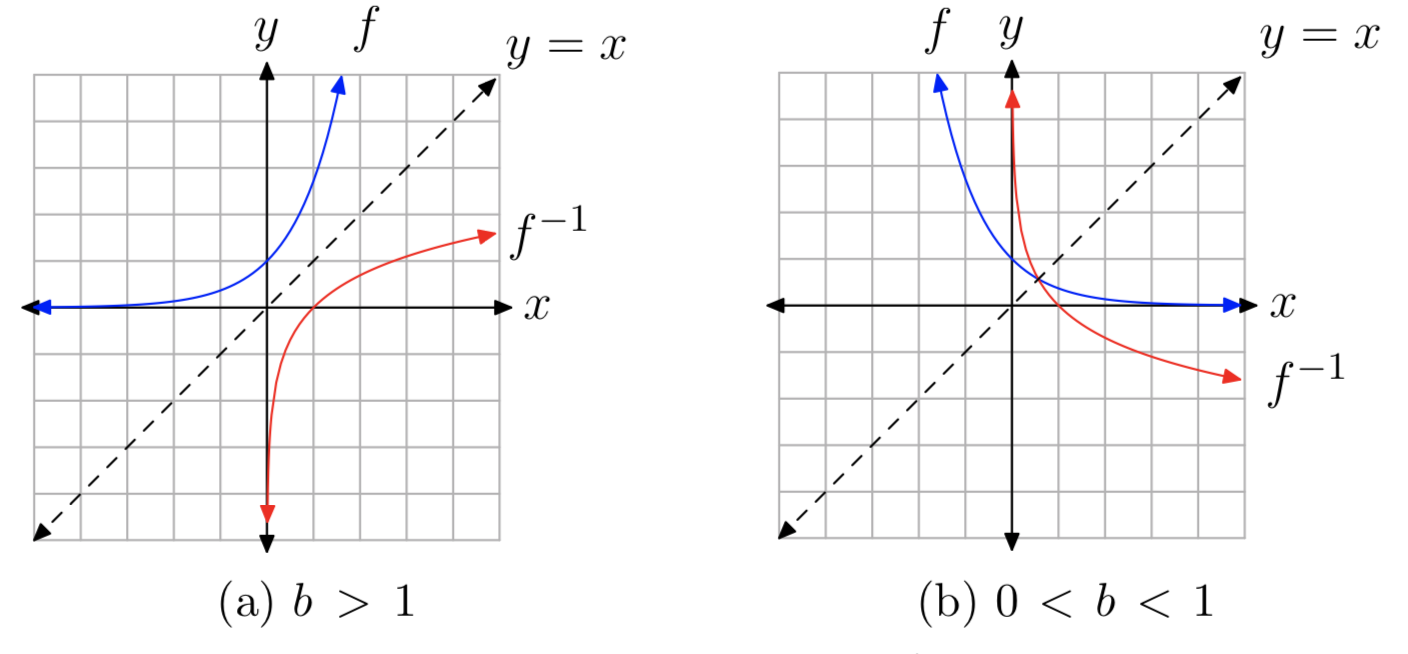
Because domains and ranges of inverse functions are interchanged, it follows that

PROPERTY $\PageIndex{16}$

$Domain(log_{b}(x)) = (0, \infty)$

and

$Range(log_{b}(x)) = (−\infty, \infty)$.

In particular, note that the logarithm of a negative number, as well as the logarithm of 0, are not defined.

Two particular points on the graph of the logarithm are noteworthy. Since $b^0 = 1$, it follows that $log_{b}(1) = 0$, and therefore the x-intercept of the graph of $log_{b}(x)$ is (1, 0). Similarly, since $b^1 = b$, it follows that $log_{b}(b) = 1$, and therefore (b, 1) is on the graph.

PROPERTY $\PageIndex{17}$

$log_{b}(1) = 0$

and

$log_{b}(b) = 1$

Finally, since the graph of $b^x$ has a horizontal asymptote y = 0, the graph of $log_{b}(x)$ must have a vertical asymptote x = 0. This behavior is a consequence of the fact that inputs and outputs of inverse functions are interchanged, and can be observed in Figure 4.

In the final example below, we’ll apply a transformation to the logarithm and see how that affects the graph.

Example $\PageIndex{18}$

Plot the graph of the function $f(x) = log_{2}(x+1)$.

Answer

The graph of $f(x) = log_{2}(x+1)$ will be the same as the graph of $g(x) = log_{2}(x)$ shifted one unit to the left. The graph of g is shown in Figure 1(b). The x-intercept (1, 0) on the graph of g will be shifted one unit to the left to (0,0) on the graph of f. Likewise, the vertical asymptote x = 0 on the graph of g will be shifted one unit to the left to the line x = −1 on the graph of f. The final graph of f is shown in Figure 5.

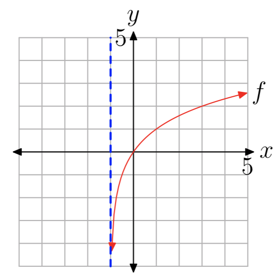
Figure 5. The graph of $f(x) = log_{2}(x+1)$.

Exercise

In Exercises 1-18, find the exact value of the function at the given value b.

Exercise $\PageIndex{1}$

$f(x) = log_{3}(x)$; $b = \sqrt[5]{3}$.

Answer

$\frac{1}{5}$

Exercise $\PageIndex{2}$

$f(x) = log_{5}(x)$; b = 3125.

Exercise $\PageIndex{3}$

$f(x) = log_{2}(x)$; $b = \frac{1}{16}$.

Answer

−4

Exercise $\PageIndex{4}$

$f(x) = log_{2}(x)$; b = 4.

Exercise $\PageIndex{5}$

$f(x) = log_{5}(x)$; b = 5.

Answer

1

Exercise $\PageIndex{6}$

$f(x) = log_{2}(x)$; b = 8.

Exercise $\PageIndex{7}$

$f(x) = log_{2}(x)$; b = 32.

Answer

5

Exercise $\PageIndex{8}$

$f(x) = log_{4}(x)$; $b = \frac{1}{16}$.

Exercise $\PageIndex{9}$

$f(x) = log_{5}(x)$; $b = \frac{1}{3125}$.

Answer

−5

Exercise $\PageIndex{10}$

$f(x) = log_{5}(x)$; $b = \frac{1}{25}$.

Exercise $\PageIndex{11}$

$f(x) = log_{5}(x)$; $b = \sqrt[6]{5}$.

Answer

$\frac{1}{6}$

Exercise $\PageIndex{12}$

$f(x) = log_{3}(x)$; $b = \sqrt[3]{3}$.

Exercise $\PageIndex{13}$

$f(x) = log_{6}(x)$; $b = \sqrt[6]{6}$.

Answer

$\frac{1}{6}$

Exercise $\PageIndex{14}$

$f(x) = log_{5}(x)$; $b = \sqrt[5]{5}$.

Exercise $\PageIndex{15}$

$f(x) = log_{2}(x)$; $b = \sqrt[6]{2}$.

Answer

$\frac{1}{6}$

Exercise $\PageIndex{16}$

$f(x) = log_{4}(x)$; $b = \frac{1}{4}$.

Exercise $\PageIndex{17}$

$f(x) = log_{3}(x)$; $b = \frac{1}{9}$.

Answer

−2

Exercise $\PageIndex{18}$

$f(x) = log_{4}(x)$; b = 64.

​​​​​​In Exercises 19-26, use a calculator to evaluate the function at the given value p. Round your answer to the nearest hundredth.

Exercise $\PageIndex{19}$

f(x) = ln(x); p = 10.06.

Answer

2.31

Exercise $\PageIndex{20}$

f(x) = ln(x); p = 9.87.

Exercise $\PageIndex{21}$

f(x) = ln(x); p = 2.40.

Answer

0.88

Exercise $\PageIndex{22}$

f(x) = ln(x); p = 9.30.

Exercise $\PageIndex{23}$

f(x) = log(x); p = 7.68.

Answer

0.89

Exercise $\PageIndex{24}$

f(x) = log(x); p = 652.22.

Exercise $\PageIndex{25}$

f(x) = log(x); p = 6.47.

Answer

0.81

Exercise $\PageIndex{26}$

f(x) = log(x); p = 86.19.

In Exercises 27-34, solve the given equation, and round your answer to the nearest hundredth.

Exercise $\PageIndex{27}$

$13 = e^{8x}$

Answer

0.32

Exercise $\PageIndex{28}$

$2 = 8e^{x}$

Exercise $\PageIndex{29}$

$19 = 10^{8x}$

Answer

0.16

Exercise $\PageIndex{30}$

$17 = 10^{2x}$

Exercise $\PageIndex{31}$

$7 = 6(10)^{x}$

Answer

0.07

Exercise $\PageIndex{32}$

$7 = e^{9x}$

Exercise $\PageIndex{33}$

$13 = 8e^{x}$

Answer

0.49

Exercise $\PageIndex{34}$

$5 = 7(10)^{x}$

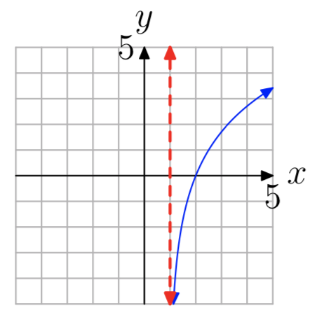
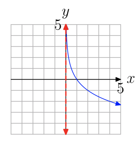
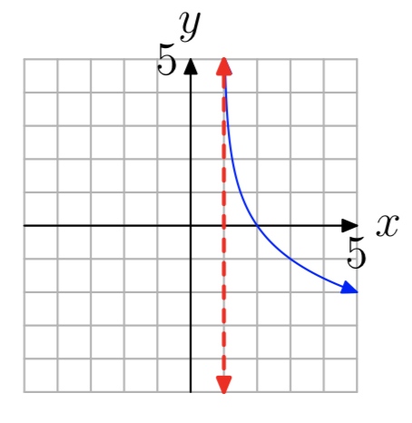
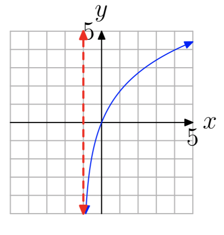
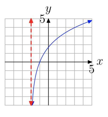
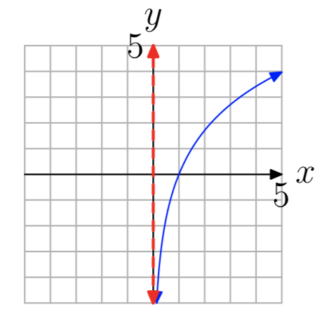
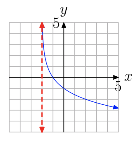
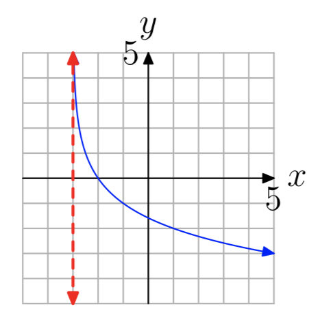
In Exercises 35-42, the graph of a logarithmic function of the form $f(x) = log_{b}(x−a)$ is shown. The dashed red line is a vertical asymptote. Determine the domain of the function. Express your answer in interval notation.

Exercise $\PageIndex{35}$

Answer

$(0, \infty)$

Exercise $\PageIndex{36}$

Exercise $\PageIndex{37}$

Answer

$(−1, \infty)$

Exercise $\PageIndex{38}$

Exercise $\PageIndex{39}$

Answer

$(0, \infty)$

Exercise $\PageIndex{40}$

Exercise $\PageIndex{41}$

Answer

$(−3, \infty)$

Exercise $\PageIndex{42}$