
7.2: Systems of Linear Equations - Two Variables
- Page ID
- 15087

\( \newcommand{\vecs}[1]{\overset { \scriptstyle \rightharpoonup} {\mathbf{#1}} } \)
\( \newcommand{\vecd}[1]{\overset{-\!-\!\rightharpoonup}{\vphantom{a}\smash {#1}}} \)
\( \newcommand{\dsum}{\displaystyle\sum\limits} \)
\( \newcommand{\dint}{\displaystyle\int\limits} \)
\( \newcommand{\dlim}{\displaystyle\lim\limits} \)
\( \newcommand{\id}{\mathrm{id}}\) \( \newcommand{\Span}{\mathrm{span}}\)
( \newcommand{\kernel}{\mathrm{null}\,}\) \( \newcommand{\range}{\mathrm{range}\,}\)
\( \newcommand{\RealPart}{\mathrm{Re}}\) \( \newcommand{\ImaginaryPart}{\mathrm{Im}}\)
\( \newcommand{\Argument}{\mathrm{Arg}}\) \( \newcommand{\norm}[1]{\| #1 \|}\)
\( \newcommand{\inner}[2]{\langle #1, #2 \rangle}\)
\( \newcommand{\Span}{\mathrm{span}}\)
\( \newcommand{\id}{\mathrm{id}}\)
\( \newcommand{\Span}{\mathrm{span}}\)
\( \newcommand{\kernel}{\mathrm{null}\,}\)
\( \newcommand{\range}{\mathrm{range}\,}\)
\( \newcommand{\RealPart}{\mathrm{Re}}\)
\( \newcommand{\ImaginaryPart}{\mathrm{Im}}\)
\( \newcommand{\Argument}{\mathrm{Arg}}\)
\( \newcommand{\norm}[1]{\| #1 \|}\)
\( \newcommand{\inner}[2]{\langle #1, #2 \rangle}\)
\( \newcommand{\Span}{\mathrm{span}}\) \( \newcommand{\AA}{\unicode[.8,0]{x212B}}\)
\( \newcommand{\vectorA}[1]{\vec{#1}} % arrow\)
\( \newcommand{\vectorAt}[1]{\vec{\text{#1}}} % arrow\)
\( \newcommand{\vectorB}[1]{\overset { \scriptstyle \rightharpoonup} {\mathbf{#1}} } \)
\( \newcommand{\vectorC}[1]{\textbf{#1}} \)
\( \newcommand{\vectorD}[1]{\overrightarrow{#1}} \)
\( \newcommand{\vectorDt}[1]{\overrightarrow{\text{#1}}} \)
\( \newcommand{\vectE}[1]{\overset{-\!-\!\rightharpoonup}{\vphantom{a}\smash{\mathbf {#1}}}} \)
\( \newcommand{\vecs}[1]{\overset { \scriptstyle \rightharpoonup} {\mathbf{#1}} } \)
\(\newcommand{\longvect}{\overrightarrow}\)
\( \newcommand{\vecd}[1]{\overset{-\!-\!\rightharpoonup}{\vphantom{a}\smash {#1}}} \)
\(\newcommand{\avec}{\mathbf a}\) \(\newcommand{\bvec}{\mathbf b}\) \(\newcommand{\cvec}{\mathbf c}\) \(\newcommand{\dvec}{\mathbf d}\) \(\newcommand{\dtil}{\widetilde{\mathbf d}}\) \(\newcommand{\evec}{\mathbf e}\) \(\newcommand{\fvec}{\mathbf f}\) \(\newcommand{\nvec}{\mathbf n}\) \(\newcommand{\pvec}{\mathbf p}\) \(\newcommand{\qvec}{\mathbf q}\) \(\newcommand{\svec}{\mathbf s}\) \(\newcommand{\tvec}{\mathbf t}\) \(\newcommand{\uvec}{\mathbf u}\) \(\newcommand{\vvec}{\mathbf v}\) \(\newcommand{\wvec}{\mathbf w}\) \(\newcommand{\xvec}{\mathbf x}\) \(\newcommand{\yvec}{\mathbf y}\) \(\newcommand{\zvec}{\mathbf z}\) \(\newcommand{\rvec}{\mathbf r}\) \(\newcommand{\mvec}{\mathbf m}\) \(\newcommand{\zerovec}{\mathbf 0}\) \(\newcommand{\onevec}{\mathbf 1}\) \(\newcommand{\real}{\mathbb R}\) \(\newcommand{\twovec}[2]{\left[\begin{array}{r}#1 \\ #2 \end{array}\right]}\) \(\newcommand{\ctwovec}[2]{\left[\begin{array}{c}#1 \\ #2 \end{array}\right]}\) \(\newcommand{\threevec}[3]{\left[\begin{array}{r}#1 \\ #2 \\ #3 \end{array}\right]}\) \(\newcommand{\cthreevec}[3]{\left[\begin{array}{c}#1 \\ #2 \\ #3 \end{array}\right]}\) \(\newcommand{\fourvec}[4]{\left[\begin{array}{r}#1 \\ #2 \\ #3 \\ #4 \end{array}\right]}\) \(\newcommand{\cfourvec}[4]{\left[\begin{array}{c}#1 \\ #2 \\ #3 \\ #4 \end{array}\right]}\) \(\newcommand{\fivevec}[5]{\left[\begin{array}{r}#1 \\ #2 \\ #3 \\ #4 \\ #5 \\ \end{array}\right]}\) \(\newcommand{\cfivevec}[5]{\left[\begin{array}{c}#1 \\ #2 \\ #3 \\ #4 \\ #5 \\ \end{array}\right]}\) \(\newcommand{\mattwo}[4]{\left[\begin{array}{rr}#1 \amp #2 \\ #3 \amp #4 \\ \end{array}\right]}\) \(\newcommand{\laspan}[1]{\text{Span}\{#1\}}\) \(\newcommand{\bcal}{\cal B}\) \(\newcommand{\ccal}{\cal C}\) \(\newcommand{\scal}{\cal S}\) \(\newcommand{\wcal}{\cal W}\) \(\newcommand{\ecal}{\cal E}\) \(\newcommand{\coords}[2]{\left\{#1\right\}_{#2}}\) \(\newcommand{\gray}[1]{\color{gray}{#1}}\) \(\newcommand{\lgray}[1]{\color{lightgray}{#1}}\) \(\newcommand{\rank}{\operatorname{rank}}\) \(\newcommand{\row}{\text{Row}}\) \(\newcommand{\col}{\text{Col}}\) \(\renewcommand{\row}{\text{Row}}\) \(\newcommand{\nul}{\text{Nul}}\) \(\newcommand{\var}{\text{Var}}\) \(\newcommand{\corr}{\text{corr}}\) \(\newcommand{\len}[1]{\left|#1\right|}\) \(\newcommand{\bbar}{\overline{\bvec}}\) \(\newcommand{\bhat}{\widehat{\bvec}}\) \(\newcommand{\bperp}{\bvec^\perp}\) \(\newcommand{\xhat}{\widehat{\xvec}}\) \(\newcommand{\vhat}{\widehat{\vvec}}\) \(\newcommand{\uhat}{\widehat{\uvec}}\) \(\newcommand{\what}{\widehat{\wvec}}\) \(\newcommand{\Sighat}{\widehat{\Sigma}}\) \(\newcommand{\lt}{<}\) \(\newcommand{\gt}{>}\) \(\newcommand{\amp}{&}\) \(\definecolor{fillinmathshade}{gray}{0.9}\)- Solve systems of equations by graphing.
- Solve systems of equations by substitution.
- Solve systems of equations by addition.
- Identify inconsistent systems of equations containing two variables.
- Express the solution of a system of dependent equations containing two variables.
A skateboard manufacturer introduces a new line of boards. The manufacturer tracks its costs, which is the amount it spends to produce the boards, and its revenue, which is the amount it earns through sales of its boards. How can the company determine if it is making a profit with its new line? How many skateboards must be produced and sold before a profit is possible? In this section, we will consider linear equations with two variables to answer these and similar questions.

Introduction to Systems of Equations
In order to investigate situations such as that of the skateboard manufacturer, we need to recognize that we are dealing with more than one variable and likely more than one equation. A system of linear equations consists of two or more linear equations made up of two or more variables such that all equations in the system are considered simultaneously. To find the unique solution to a system of linear equations, we must find a numerical value for each variable in the system that will satisfy all equations in the system at the same time. Some linear systems may not have a solution and others may have an infinite number of solutions. In order for a linear system to have a unique solution, there must be at least as many equations as there are variables. Even so, this does not guarantee a unique solution.
In this section, we will look at systems of linear equations in two variables, which consist of two equations that contain two different variables. For example, consider the following system of linear equations in two variables.
\[\begin{align*} 2x+y &= 15 \\ 3x–y &= 5 \end{align*}\]
The solution to a system of linear equations in two variables is any ordered pair that satisfies each equation independently. In this example, the ordered pair \((4,7)\) is the solution to the system of linear equations. We can verify the solution by substituting the values into each equation to see if the ordered pair satisfies both equations. Shortly we will investigate methods of finding such a solution if it exists.
\[\begin{align*} 2(4)+(7) &=15 \text{ True} \\ 3(4)−(7) &= 5 \text{ True} \end{align*}\]
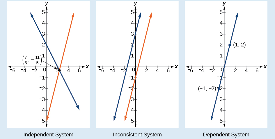
In addition to considering the number of equations and variables, we can categorize systems of linear equations by the number of solutions. A consistent system of equations has at least one solution. A consistent system is considered to be an independent system if it has a single solution, such as the example we just explored. The two lines have different slopes and intersect at one point in the plane. A consistent system is considered to be a dependent system if the equations have the same slope and the same y-intercepts. In other words, the lines coincide so the equations represent the same line. Every point on the line represents a coordinate pair that satisfies the system. Thus, there are an infinite number of solutions.
Another type of system of linear equations is an inconsistent system, which is one in which the equations represent two parallel lines. The lines have the same slope and different y-intercepts. There are no points common to both lines; hence, there is no solution to the system.
There are three types of systems of linear equations in two variables, and three types of solutions.
- An independent system has exactly one solution pair \((x,y)\). The point where the two lines intersect is the only solution.
- An inconsistent system has no solution. Notice that the two lines are parallel and will never intersect.
- A dependent system has infinitely many solutions. The lines are coincident. They are the same line, so every coordinate pair on the line is a solution to both equations.
Figure \(\PageIndex{2}\) compares graphical representations of each type of system.
- Substitute the ordered pair into each equation in the system.
- Determine whether true statements result from the substitution in both equations; if so, the ordered pair is a solution.
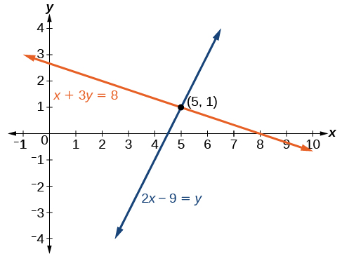
Determine whether the ordered pair \((5,1)\) is a solution to the given system of equations.
\[\begin{align*} x+3y &= 8 \\ 2x−9 &= y \end{align*}\]
Solution
Substitute the ordered pair \((5,1)\) into both equations.
\[ \begin{align*} (5)+3(1) &= 8 \\ 8 &= 8 \text{ True} \\ 2(5)−9 &= (1) \\ 1 &= 1 \text{ True} \end{align*}\]
The ordered pair \((5,1)\) satisfies both equations, so it is the solution to the system.
Analysis
We can see the solution clearly by plotting the graph of each equation. Since the solution is an ordered pair that satisfies both equations, it is a point on both of the lines and thus the point of intersection of the two lines. See Figure \(\PageIndex{3}\).
Determine whether the ordered pair \((8,5)\) is a solution to the following system.
\[\begin{align*} 5x−4y &= 20 \\ 2x+1 &= 3y \end{align*}\]
- Answer
-
Not a solution.
Solving Systems of Equations by Graphing
There are multiple methods of solving systems of linear equations. For a system of linear equations in two variables, we can determine both the type of system and the solution by graphing the system of equations on the same set of axes.
Solve the following system of equations by graphing. Identify the type of system.
\[\begin{align*} 2x+y &= −8 \\ x−y &= −1 \end{align*}\]
Solution
Solve the first equation for \(y\).
\[\begin{align*} 2x+y &= −8 \\ y &= −2x−8 \end{align*}\]
Solve the second equation for \(y\).
\[\begin{align*} x−y &= −1 \\ y &= x+1 \end{align*}\]
Graph both equations on the same set of axes as in Figure \(\PageIndex{4}\).
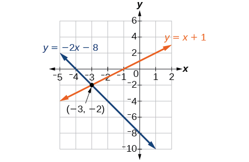
The lines appear to intersect at the point \((−3,−2)\). We can check to make sure that this is the solution to the system by substituting the ordered pair into both equations.
\[\begin{align*} 2(−3)+(−2) &= −8 \\ −8 &= −8 \text{ True} \\ (−3)−(−2) &= −1 \\ −1 &= −1 \text{ True} \end{align*}\]
The solution to the system is the ordered pair \((−3,−2)\),so the system is independent.
Solve the following system of equations by graphing.
\[\begin{align*} 2x−5y &= −25 \\ −4x+5y &= 35 \end{align*}\]
- Answer
-
The solution to the system is the ordered pair \((−5,3)\).
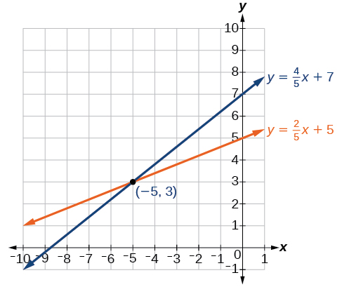
Figure \(\PageIndex{5}\)
Can graphing be used if the system is inconsistent or dependent?
Yes, in both cases we can still graph the system to determine the type of system and solution. If the two lines are parallel, the system has no solution and is inconsistent. If the two lines are identical, the system has infinite solutions and is a dependent system.
Solving Systems of Equations by Substitution
Solving a linear system in two variables by graphing works well when the solution consists of integer values, but if our solution contains decimals or fractions, it is not the most precise method. We will consider two more methods of solving a system of linear equations that are more precise than graphing. One such method is solving a system of equations by the substitution method, in which we solve one of the equations for one variable and then substitute the result into the second equation to solve for the second variable. Recall that we can solve for only one variable at a time, which is the reason the substitution method is both valuable and practical.
- Solve one of the two equations for one of the variables in terms of the other.
- Substitute the expression for this variable into the second equation, then solve for the remaining variable.
- Substitute that solution into either of the original equations to find the value of the first variable. If possible, write the solution as an ordered pair.
- Check the solution in both equations.
Solve the following system of equations by substitution.
\[\begin{align*} −x+y &= −5 \\ 2x−5y &= 1 \end{align*}\]
Solution
First, we will solve the first equation for \(y\).
\[\begin{align*} −x+y &=−5 \\ y &= x−5 \end{align*}\]
Now we can substitute the expression \(x−5\) for \(y\) in the second equation.
\[\begin{align*} 2x−5y &= 1 \\ 2x−5(x−5) &= 1 \\ 2x−5x+25 &= 1 \\ −3x &= −24 \\ x &= 8 \end{align*}\]
Now, we substitute \(x=8\) into the first equation and solve for \(y\).
\[\begin{align*} −(8)+y &= −5 \\ y &= 3 \end{align*}\]
Our solution is \((8,3)\).
Check the solution by substituting \((8,3)\) into both equations.
\[\begin{align*} −x+y &= −5 \\ −(8)+(3) &= −5 \text{ True} \\ 2x−5y &= 1 \\ 2(8)−5(3) &= 1 \text{ True} \end{align*}\]
Solve the following system of equations by substitution.
\[\begin{align*} x &= y+3 \\ 4 &= 3x−2y \end{align*}\]
- Answer
-
\((−2,−5)\)
Can the substitution method be used to solve any linear system in two variables?
Yes, but the method works best if one of the equations contains a coefficient of \(1\) or \(–1\) so that we do not have to deal with fractions.
Solving Systems of Equations in Two Variables by the Addition Method
A third method of solving systems of linear equations is the addition method. In this method, we add two terms with the same variable, but opposite coefficients, so that the sum is zero. Of course, not all systems are set up with the two terms of one variable having opposite coefficients. Often we must adjust one or both of the equations by multiplication so that one variable will be eliminated by addition.
- Write both equations with x- and y-variables on the left side of the equal sign and constants on the right.
- Write one equation above the other, lining up corresponding variables. If one of the variables in the top equation has the opposite coefficient of the same variable in the bottom equation, add the equations together, eliminating one variable. If not, use multiplication by a nonzero number so that one of the variables in the top equation has the opposite coefficient of the same variable in the bottom equation, then add the equations to eliminate the variable.
- Solve the resulting equation for the remaining variable.
- Substitute that value into one of the original equations and solve for the second variable.
- Check the solution by substituting the values into the other equation.
Solve the given system of equations by addition.
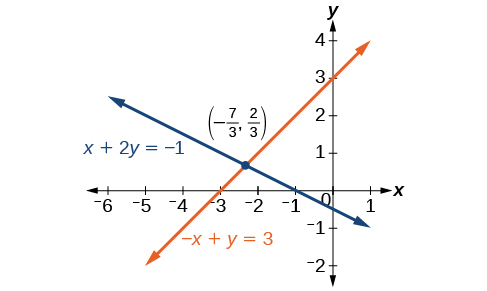
\[\begin{align*} x+2y &= −1 \\ −x+y &=3 \end{align*}\]
Solution
Both equations are already set equal to a constant. Notice that the coefficient of \(x\) in the second equation, \(–1\), is the opposite of the coefficient of \(x\) in the first equation, \(1\). We can add the two equations to eliminate \(x\) without needing to multiply by a constant.
\[\begin{align*} x+2y &= -1 \\ \underline{-x+y}& = \underline{3} \\ 3y&= 2 \\ \end{align*}\]
Now that we have eliminated \(x\), we can solve the resulting equation for \(y\).
\[\begin{align*} 3y &= 2 \\ y &=\dfrac{2}{3} \end{align*}\]
Then, we substitute this value for \(y\) into one of the original equations and solve for \(x\).
\[\begin{align*} −x+y &= 3 \\ −x+\dfrac{2}{3} &= 3 \\ −x &= 3−\dfrac{2}{3} \\ −x &= \dfrac{7}{3} \\ x &= −\dfrac{7}{3} \end{align*}\]
The solution to this system is \(\left(−\dfrac{7}{3},\dfrac{2}{3}\right)\).
Check the solution in the first equation.
\[\begin{align*} x+2y &= −1 \\ \left(−\dfrac{7}{3}\right)+2\left(\dfrac{2}{3}\right) &= \\ −\dfrac{7}{3}+\dfrac{4}{3} &= −\dfrac{3}{3} \\ −1 &= −1 \;\;\;\;\;\;\;\; \text{True} \end{align*}\]
Analysis
We gain an important perspective on systems of equations by looking at the graphical representation. See Figure \(\PageIndex{6}\) to find that the equations intersect at the solution. We do not need to ask whether there may be a second solution because observing the graph confirms that the system has exactly one solution.
Solve the given system of equations by the addition method.
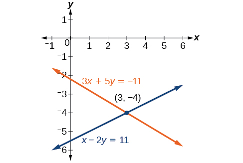
\[\begin{align*} 3x+5y &= −11 \\ x−2y &= 11 \end{align*}\]
Solution
Adding these equations as presented will not eliminate a variable. However, we see that the first equation has \(3x\) in it and the second equation has \(x\). So if we multiply the second equation by \(−3\),the x-terms will add to zero.
\[\begin{align*} x−2y &= 11 \\ −3(x−2y) &=−3(11) \;\;\;\;\;\;\;\; \text{Multiply both sides by }−3. \\ −3x+6y &= −33 \;\;\;\;\;\;\;\;\; \text{Use the distributive property.} \end{align*}\]
Now, let’s add them.
\[\begin{align*} 3x+5y &= -11 \\ \underline{-3x+6y }& = \underline{-33} \\ 11y&= -44 \\ y&= -4 \end{align*}\]
For the last step, we substitute \(y=−4\) into one of the original equations and solve for \(x\).
\[\begin{align*} 3x+5y &= −11 \\ 3x+5(−4) &= −11 \\ 3x−20 &= −11 \\ 3x &= 9 \\ x &= 3 \end{align*}\]
Our solution is the ordered pair \((3,−4)\). See Figure \(\PageIndex{7}\). Check the solution in the original second equation.
\[\begin{align*} x−2y &= 11 \\ (3)−2(−4) &= 3+8 \\ &= 11 \;\;\;\;\;\;\;\;\;\; \text{True} \end{align*}\]
Solve the system of equations by addition.
\[\begin{align*} 2x−7y &= 2 \\ 3x+y &= −20 \end{align*}\]
- Answer
-
\((−6,−2)\)
Solve the given system of equations in two variables by addition.
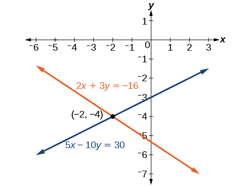
\[\begin{align*} 2x+3y &= −16 \\ 5x−10y &= 30 \end{align*}\]
Solution
One equation has \(2x\) and the other has \(5x\). The least common multiple is \(10x\) so we will have to multiply both equations by a constant in order to eliminate one variable. Let’s eliminate \(x\) by multiplying the first equation by \(−5\) and the second equation by \(2\).
\[\begin{align*} −5(2x+3y) &= −5(−16) \\ −10x−15y &= 80 \\ 2(5x−10y) &= 2(30) \\ 10x−20y &= 60 \end{align*}\]
Then, we add the two equations together.
\[\begin{align*} -10x-15y &= 80 \\ \underline{10x-20y}& = \underline{60} \\ -35y&= 140 \\ y&= -4 \end{align*}\]
Substitute \(y=−4\) into the original first equation.
\[ \begin{align*} 2x+3(−4) &=−16 \\ 2x−12 &= −16 \\ 2x &= −4 \\ x &=−2 \end{align*}\]
The solution is \((−2,−4)\). Check it in the other equation.
\[\begin{align*} 5x−10y &= 30 \\ 5(−2)−10(−4) &= 30 \\ −10+40 &= 30 \\30 &=30 \end{align*}\]
See Figure \(\PageIndex{8}\).
Solve the given system of equations in two variables by addition.
\[ \begin{align*} \dfrac{x}{3}+\dfrac{y}{6} &= 3 \\ \dfrac{x}{2}−\dfrac{y}{4} &= 1 \end{align*}\]
Solution
First clear each equation of fractions by multiplying both sides of the equation by the least common denominator.
\[\begin{align*} 6\left(\dfrac{x}{3}+\dfrac{y}{6}\right) &= 6(3) \\ 2x+y &= 18 \\ 4\left(\dfrac{x}{2}−\dfrac{y}{4}\right) &= 4(1) \\ 2x−y &= 4 \end{align*}\]
Now multiply the second equation by \(−1\) so that we can eliminate the x-variable.
\[\begin{align*} −1(2x−y) &= −1(4) \\ −2x+y &= −4 \end{align*}\]
Add the two equations to eliminate the \(x\)-variable and solve the resulting equation.
\[\begin{align*} 2x+y &= 18 \\ −2x+y &= −4 \\ 2y &= 14 \\ y &=7 \end{align*}\]
Substitute \(y=7\) into the first equation.
\[\begin{align*} 2x+(7) &= 18 \\ 2x &= 11 \\ x &= \dfrac{11}{2} \\ &= 7.5 \end{align*}\]
The solution is \(\left(\dfrac{11}{2},7\right)\). Check it in the other equation.
\[\begin{align*} \dfrac{x}{2}−\dfrac{y}{4} &= 1 \\ \dfrac{\dfrac{11}{2}}{2}−\dfrac{7}{4} &=1 \\ \dfrac{11}{4}−\dfrac{7}{4} &=1 \\ \dfrac{4}{4} &=1 \end{align*}\]
Solve the system of equations by addition.
\[\begin{align*} 2x+3y &= 8 \\ 3x+5y &= 10 \end{align*}\]
- Answer
-
\((10,−4)\)
Identifying Inconsistent Systems of Equations Containing Two Variables
Now that we have several methods for solving systems of equations, we can use the methods to identify inconsistent systems. Recall that an inconsistent system consists of parallel lines that have the same slope but different y-intercepts. They will never intersect. When searching for a solution to an inconsistent system, we will come up with a false statement, such as \(12=0\).
Solve the following system of equations.
\[\begin{align*} x &= 9−2y \\ x+2y &= 13 \end{align*}\]
Solution
We can approach this problem in two ways. Because one equation is already solved for \(x\), the most obvious step is to use substitution.
\[\begin{align*} x+2y &= 13 \\ (9−2y)+2y &= 13 \\ 9+0y &= 13 \\ 9 &= 13 \end{align*}\]
Clearly, this statement is a contradiction because \(9≠13\). Therefore, the system has no solution.
The second approach would be to first manipulate the equations so that they are both in slope-intercept form. We manipulate the first equation as follows.
\[\begin{align*} x &= 9−2y \\ 2y &= −x+9 \\ y &= −\dfrac{1}{2}x+\dfrac{9}{2} \end{align*}\]
We then convert the second equation expressed to slope-intercept form.
\[\begin{align*} x+2y &= 13 \\ 2y &= −x+13 \\ y &= −\dfrac{1}{2}x+\dfrac{13}{2} \end{align*}\]
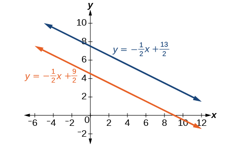
Comparing the equations, we see that they have the same slope but different \(y\)-intercepts. Therefore, the lines are parallel and do not intersect.
\[\begin{align*} y &= −\dfrac{1}{2}x+\dfrac{9}{2} \\ y &= −\dfrac{1}{2}x+\dfrac{13}{2} \end{align*}\]
Analysis
Writing the equations in slope-intercept form confirms that the system is inconsistent because all lines will intersect eventually unless they are parallel. Parallel lines will never intersect; thus, the two lines have no points in common. The graphs of the equations in this example are shown in Figure \(\PageIndex{9}\).
Solve the following system of equations in two variables.
\[\begin{align*} 2y−2x &= 2 \\ 2y−2x &= 6 \end{align*}\]
- Answer
-
No solution. It is an inconsistent system.
Expressing the Solution of a System of Dependent Equations Containing Two Variables
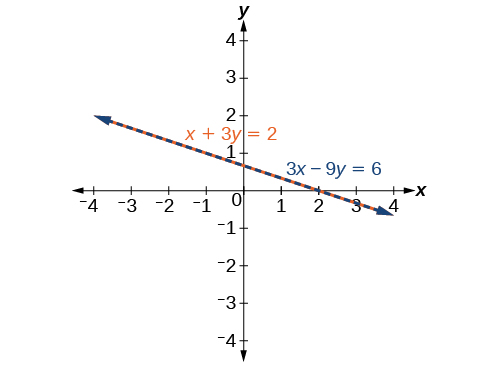
Recall that a dependent system of equations in two variables is a system in which the two equations represent the same line. Dependent systems have an infinite number of solutions because all of the points on one line are also on the other line. After using substitution or addition, the resulting equation will be an identity, such as \(0=0\).
Find a solution to the system of equations using the addition method.
\[\begin{align*} x+3y &= 2 \\ 3x+9y &= 6 \end{align*}\]
Solution
With the addition method, we want to eliminate one of the variables by adding the equations. In this case, let’s focus on eliminating \(x\). If we multiply both sides of the first equation by \(−3\), then we will be able to eliminate the x-variable.
\[\begin{align*} x+3y &= 2 \\ (−3)(x+3y) &= (−3)(2) \\ −3x−9y &= −6 \end{align*}\]
Now add the equations.
\[\begin{align*} -3x-9y &= -6 \\ \underline{+\space 3x+9y}& = \underline{6} \\ 0&= 0 \\ \end{align*}\]
We can see that there will be an infinite number of solutions that satisfy both equations.
Analysis
If we rewrote both equations in the slope-intercept form, we might know what the solution would look like before adding. Let’s look at what happens when we convert the system to slope-intercept form.
\[ \begin{align*} x+3y &= 2 \\ 3y &= −x+2 \\ y &= −\dfrac{1}{3}x+\dfrac{2}{3} \\ 3x+9y &= 6 \\ 9y &=−3x+6 \\ y &= −\dfrac{3}{9}x+\dfrac{6}{9} \\ y &= −\dfrac{1}{3}x+\dfrac{2}{3} \end{align*}\]
See Figure \(\PageIndex{10}\). Notice the results are the same. The general solution to the system is \(\left(x, −\dfrac{1}{3}x+\dfrac{2}{3}\right)\).
Solve the following system of equations in two variables.
\[\begin{align*} y−2x &= 5 \\ −3y+6x &= −15 \end{align*}\]
- Answer
-
The system is dependent so there are infinite solutions of the form \((x,2x+5)\).
Using Systems of Equations to Investigate Profits
Using what we have learned about systems of equations, we can return to the skateboard manufacturing problem at the beginning of the section. The skateboard manufacturer’s revenue function is the function used to calculate the amount of money that comes into the business. It can be represented by the equation \(R=xp\), where \(x\)=quantity and \(p\)=price. The revenue function is shown in orange in Figure \(\PageIndex{11}\).
The cost function is the function used to calculate the costs of doing business. It includes fixed costs, such as rent and salaries, and variable costs, such as utilities. The cost function is shown in blue in Figure \(\PageIndex{11}\). The \(x\)-axis represents quantity in hundreds of units. The \(y\)-axis represents either cost or revenue in hundreds of dollars.
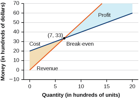
The point at which the two lines intersect is called the break-even point. We can see from the graph that if \(700\) units are produced, the cost is \($3,300\) and the revenue is also \($3,300\). In other words, the company breaks even if they produce and sell \(700\) units. They neither make money nor lose money.
The shaded region to the right of the break-even point represents quantities for which the company makes a profit. The shaded region to the left represents quantities for which the company suffers a loss. The profit function is the revenue function minus the cost function, written as \(P(x)=R(x)−C(x)\). Clearly, knowing the quantity for which the cost equals the revenue is of great importance to businesses.
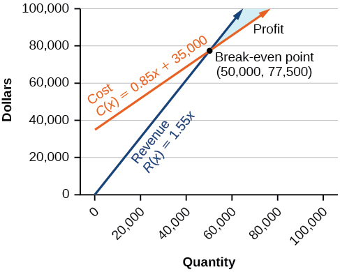
Given the cost function \(C(x)=0.85x+35,000\) and the revenue function \(R(x)=1.55x\), find the break-even point and the profit function.
Solution
Write the system of equations using \(y\) to replace function notation.
\[\begin{align*} y &= 0.85x+35,000 \\ y &= 1.55x \end{align*}\]
Substitute the expression \(0.85x+35,000\) from the first equation into the second equation and solve for \(x\).
\[\begin{align*} 0.85x+35,000 &= 1.55x \\ 35,000 &= 0.7x \\ 50,000 &= x \end{align*}\]
Then, we substitute \(x=50,000\) into either the cost function or the revenue function.
\(1.55(50,000)=77,500\)
The break-even point is \((50,000,77,500)\).
The profit function is found using the formula \(P(x)=R(x)−C(x)\).
\[\begin{align*} P(x) &= 1.55x−(0.85x+35,000) \\ &=0.7x−35,000 \end{align*}\]
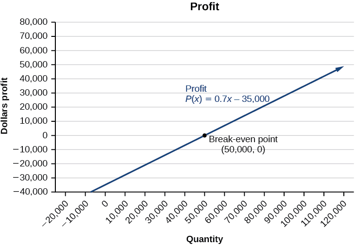
The profit function is \(P(x)=0.7x−35,000\).
Analysis
The cost to produce \(50,000\) units is \($77,500\), and the revenue from the sales of \(50,000\) units is also \($77,500\). To make a profit, the business must produce and sell more than \(50,000\) units. See Figure \(\PageIndex{12}\).
We see from the graph in Figure \(\PageIndex{13}\) that the profit function has a negative value until \(x=50,000\), when the graph crosses the \(x\)-axis. Then, the graph emerges into positive \(y\)-values and continues on this path as the profit function is a straight line. This illustrates that the break-even point for businesses occurs when the profit function is \(0\). The area to the left of the break-even point represents operating at a loss.
The cost of a ticket to the circus is \($25.00\) for children and \($50.00\) for adults. On a certain day, attendance at the circus is \(2,000\) and the total gate revenue is \($70,000\). How many children and how many adults bought tickets?
Solution
Let \(c\) = the number of children and \(a\) = the number of adults in attendance.
The total number of people is \(2,000\). We can use this to write an equation for the number of people at the circus that day.
\(c+a=2,000\)
The revenue from all children can be found by multiplying \($25.00\) by the number of children, \(25c\). The revenue from all adults can be found by multiplying \($50.00\) by the number of adults, \(50a\). The total revenue is \($70,000\). We can use this to write an equation for the revenue.
\(25c+50a=70,000\)
We now have a system of linear equations in two variables.
\(c+a=2,000\)
\(25c+50a=70,000\)
In the first equation, the coefficient of both variables is \(1\). We can quickly solve the first equation for either \(c\) or \(a\). We will solve for \(a\).
\[\begin{align*} c+a &= 2,000 \\ a &= 2,000−c \end{align*}\]
Substitute the expression \(2,000−c\) in the second equation fora a and solve for \(c\).
\[\begin{align*} 25c+50(2,000−c) &= 70,000 \\ 25c+100,000−50c &= 70,000 \\ −25c &= −30,000 \\ c &= 1,200 \end{align*}\]
Substitute \(c=1,200\) into the first equation to solve for \(a\).
\[\begin{align*} 1,200+a &= 2,000 \\ a &= 800 \end{align*}\]
We find that \(1,200\) children and \(800\) adults bought tickets to the circus that day.
Meal tickets at the circus cost \($4.00\) for children and \($12.00\) for adults. If \(1,650\) meal tickets were bought for a total of, \($14,200\), how many children and how many adults bought meal tickets?
- Answer
-
\(700\) children, \(950\) adults
Access these online resources for additional instruction and practice with systems of linear equations.
Key Concepts
- A system of linear equations consists of two or more equations made up of two or more variables such that all equations in the system are considered simultaneously.
- The solution to a system of linear equations in two variables is any ordered pair that satisfies each equation independently. See Example \(\PageIndex{1}\).
- Systems of equations are classified as independent with one solution, dependent with an infinite number of solutions, or inconsistent with no solution.
- One method of solving a system of linear equations in two variables is by graphing. In this method, we graph the equations on the same set of axes. See Example \(\PageIndex{2}\).
- Another method of solving a system of linear equations is by substitution. In this method, we solve for one variable in one equation and substitute the result into the second equation. See Example \(\PageIndex{3}\).
- A third method of solving a system of linear equations is by addition, in which we can eliminate a variable by adding opposite coefficients of corresponding variables. See Example \(\PageIndex{4}\).
- It is often necessary to multiply one or both equations by a constant to facilitate elimination of a variable when adding the two equations together. See Example \(\PageIndex{5}\), Example \(\PageIndex{6}\), and Example \(\PageIndex{7}\).
- Either method of solving a system of equations results in a false statement for inconsistent systems because they are made up of parallel lines that never intersect. See Example \(\PageIndex{8}\).
- The solution to a system of dependent equations will always be true because both equations describe the same line. See Example \(\PageIndex{9}\).
- Systems of equations can be used to solve real-world problems that involve more than one variable, such as those relating to revenue, cost, and profit. See Example \(\PageIndex{10}\) and Example \(\PageIndex{11}\).