3.3: Rates and Slope

Last updated
Save as PDF

Page ID: 19865

$ \newcommand{\vecs}[1]{\overset { \scriptstyle \rightharpoonup} {\mathbf{#1}} } $

$ \newcommand{\vecd}[1]{\overset{-\!-\!\rightharpoonup}{\vphantom{a}\smash {#1}}} $

$ \newcommand{\id}{\mathrm{id}}$ $ \newcommand{\Span}{\mathrm{span}}$

( \newcommand{\kernel}{\mathrm{null}\,}\) $ \newcommand{\range}{\mathrm{range}\,}$

$ \newcommand{\RealPart}{\mathrm{Re}}$ $ \newcommand{\ImaginaryPart}{\mathrm{Im}}$

$ \newcommand{\Argument}{\mathrm{Arg}}$ $ \newcommand{\norm}[1]{\| #1 \|}$

$ \newcommand{\inner}[2]{\langle #1, #2 \rangle}$

$ \newcommand{\Span}{\mathrm{span}}$

$ \newcommand{\id}{\mathrm{id}}$

$ \newcommand{\Span}{\mathrm{span}}$

$ \newcommand{\kernel}{\mathrm{null}\,}$

$ \newcommand{\range}{\mathrm{range}\,}$

$ \newcommand{\RealPart}{\mathrm{Re}}$

$ \newcommand{\ImaginaryPart}{\mathrm{Im}}$

$ \newcommand{\Argument}{\mathrm{Arg}}$

$ \newcommand{\norm}[1]{\| #1 \|}$

$ \newcommand{\inner}[2]{\langle #1, #2 \rangle}$

$ \newcommand{\Span}{\mathrm{span}}$ $ \newcommand{\AA}{\unicode[.8,0]{x212B}}$

$ \newcommand{\vectorA}[1]{\vec{#1}} % arrow$

$ \newcommand{\vectorAt}[1]{\vec{\text{#1}}} % arrow$

$ \newcommand{\vectorB}[1]{\overset { \scriptstyle \rightharpoonup} {\mathbf{#1}} } $

$ \newcommand{\vectorC}[1]{\textbf{#1}} $

$ \newcommand{\vectorD}[1]{\overrightarrow{#1}} $

$ \newcommand{\vectorDt}[1]{\overrightarrow{\text{#1}}} $

$ \newcommand{\vectE}[1]{\overset{-\!-\!\rightharpoonup}{\vphantom{a}\smash{\mathbf {#1}}}} $

$ \newcommand{\vecs}[1]{\overset { \scriptstyle \rightharpoonup} {\mathbf{#1}} } $

$ \newcommand{\vecd}[1]{\overset{-\!-\!\rightharpoonup}{\vphantom{a}\smash {#1}}} $

$\newcommand{\avec}{\mathbf a}$ $\newcommand{\bvec}{\mathbf b}$ $\newcommand{\cvec}{\mathbf c}$ $\newcommand{\dvec}{\mathbf d}$ $\newcommand{\dtil}{\widetilde{\mathbf d}}$ $\newcommand{\evec}{\mathbf e}$ $\newcommand{\fvec}{\mathbf f}$ $\newcommand{\nvec}{\mathbf n}$ $\newcommand{\pvec}{\mathbf p}$ $\newcommand{\qvec}{\mathbf q}$ $\newcommand{\svec}{\mathbf s}$ $\newcommand{\tvec}{\mathbf t}$ $\newcommand{\uvec}{\mathbf u}$ $\newcommand{\vvec}{\mathbf v}$ $\newcommand{\wvec}{\mathbf w}$ $\newcommand{\xvec}{\mathbf x}$ $\newcommand{\yvec}{\mathbf y}$ $\newcommand{\zvec}{\mathbf z}$ $\newcommand{\rvec}{\mathbf r}$ $\newcommand{\mvec}{\mathbf m}$ $\newcommand{\zerovec}{\mathbf 0}$ $\newcommand{\onevec}{\mathbf 1}$ $\newcommand{\real}{\mathbb R}$ $\newcommand{\twovec}[2]{\left[\begin{array}{r}#1 \\ #2 \end{array}\right]}$ $\newcommand{\ctwovec}[2]{\left[\begin{array}{c}#1 \\ #2 \end{array}\right]}$ $\newcommand{\threevec}[3]{\left[\begin{array}{r}#1 \\ #2 \\ #3 \end{array}\right]}$ $\newcommand{\cthreevec}[3]{\left[\begin{array}{c}#1 \\ #2 \\ #3 \end{array}\right]}$ $\newcommand{\fourvec}[4]{\left[\begin{array}{r}#1 \\ #2 \\ #3 \\ #4 \end{array}\right]}$ $\newcommand{\cfourvec}[4]{\left[\begin{array}{c}#1 \\ #2 \\ #3 \\ #4 \end{array}\right]}$ $\newcommand{\fivevec}[5]{\left[\begin{array}{r}#1 \\ #2 \\ #3 \\ #4 \\ #5 \\ \end{array}\right]}$ $\newcommand{\cfivevec}[5]{\left[\begin{array}{c}#1 \\ #2 \\ #3 \\ #4 \\ #5 \\ \end{array}\right]}$ $\newcommand{\mattwo}[4]{\left[\begin{array}{rr}#1 \amp #2 \\ #3 \amp #4 \\ \end{array}\right]}$ $\newcommand{\laspan}[1]{\text{Span}\{#1\}}$ $\newcommand{\bcal}{\cal B}$ $\newcommand{\ccal}{\cal C}$ $\newcommand{\scal}{\cal S}$ $\newcommand{\wcal}{\cal W}$ $\newcommand{\ecal}{\cal E}$ $\newcommand{\coords}[2]{\left\{#1\right\}_{#2}}$ $\newcommand{\gray}[1]{\color{gray}{#1}}$ $\newcommand{\lgray}[1]{\color{lightgray}{#1}}$ $\newcommand{\rank}{\operatorname{rank}}$ $\newcommand{\row}{\text{Row}}$ $\newcommand{\col}{\text{Col}}$ $\renewcommand{\row}{\text{Row}}$ $\newcommand{\nul}{\text{Nul}}$ $\newcommand{\var}{\text{Var}}$ $\newcommand{\corr}{\text{corr}}$ $\newcommand{\len}[1]{\left|#1\right|}$ $\newcommand{\bbar}{\overline{\bvec}}$ $\newcommand{\bhat}{\widehat{\bvec}}$ $\newcommand{\bperp}{\bvec^\perp}$ $\newcommand{\xhat}{\widehat{\xvec}}$ $\newcommand{\vhat}{\widehat{\vvec}}$ $\newcommand{\uhat}{\widehat{\uvec}}$ $\newcommand{\what}{\widehat{\wvec}}$ $\newcommand{\Sighat}{\widehat{\Sigma}}$ $\newcommand{\lt}{<}$ $\newcommand{\gt}{>}$ $\newcommand{\amp}{&}$ $\definecolor{fillinmathshade}{gray}{0.9}$

Let’s open this section with an application of the concept of rate.

Independent versus dependent

It is traditional to place the independent variable on the horizontal axis and the dependent variable on the vertical axis.

Example $\PageIndex{1}$

An object is dropped from rest, then begins to pick up speed at a constant rate of $10$ meters per second every second ($10(\mathrm{m} / \mathrm{s}) / \mathrm{s}$ or $10\mathrm{m} / \mathrm{s}^{2}$). Sketch the graph of the speed of the object versus time.

Solution

In this example, the speed of the object depends on the time. This makes the speed the dependent variable and time the independent variable.

Following this guideline, we place the time on the horizontal axis and the speed on the vertical axis. In Figure $\PageIndex{1}$, note that we’ve labeled each axis with the dependent and independent variables ($v$ and $t$), and we’ve included the units ($\mathrm{m} / \mathrm{s}$ and $\mathrm{s}$) in our labels. Next, we need to scale each axis. In determining a scale for each axis, keep two thoughts in mind:

Pick a scale that makes it convenient to plot the given data.
Pick a scale that allows all of the given data to fit on the graph.

In this example, we want a scale that makes it convenient to show that the speed is increasing at a rate of $10$ meters per second ($10\mathrm{m} / \mathrm{s}$) every second ($\mathrm{m} / \mathrm{s}$). One possible approach is to make each tick mark on the horizontal axis equal to $1 \mathrm{s}$ and each tick mark on the vertical axis equal to $10\mathrm{m} / \mathrm{s}$.

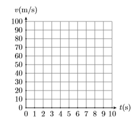
fig 3.3.1.png — Figure $\PageIndex{1}$: Label and scale each axis. Include units with labels.

Next, at time $t=0 \mathrm{s}$, the speed is $v=0 \mathrm{m} / \mathrm{s}$. This is the point $(t, v)=(0,0)$ plotted in Figure $\PageIndex{2}$. Secondly, the rate at which the speed is increasing is ($10\mathrm{m} / \mathrm{s}$) per second. This means that every time you move $1$ second to the right, the speed increases by ($10\mathrm{m} / \mathrm{s}$).

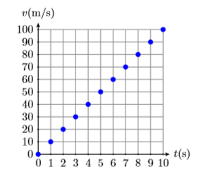
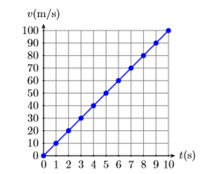
fig 3.3.2.png — Figure $\PageIndex{2}$: Start at $(0,0)$, then continuously move $1$ right and $10$ up.

In Figure $\PageIndex{2}$, start at $(0,0)$, then move $1 \mathrm{s}$ to the right and ($10\mathrm{m} / \mathrm{s}$) up. This places you at the point $(1,10)$, which says that after $1$ second, the speed of the particle is ($10\mathrm{m} / \mathrm{s}$) . Continue in this manner, continuously moving $1 \mathrm{s}$ to the right and ($10\mathrm{m} / \mathrm{s}$) upward. This produces the sequence of points shown in Figure $\PageIndex{2}$. Note that this constant rate of $10(\mathrm{m} / \mathrm{s}) / \mathrm{s}$ forces the graph of the speed versus time to be a line, as depicted in Figure $\PageIndex{3}$.

alt — Figure $\PageIndex{3}$: The constant rate forces the graph to be a line.

fig 3.3.3.png — Figure $\PageIndex{3}$: The constant rate forces the graph to be a line.

Exercise $\PageIndex{1}$

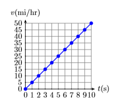
Starting from rest, an automobile picks up speed at a constant rate of $5$ miles per hour every second (5$(\mathrm{mi} / \mathrm{hr}) / \mathrm{s}$). Sketch the graph of the speed of the object versus time.

Answer: $Exercise 3.3.1.png$

Measuring the Change in a Variable

To calculate the change in some quantity, we take a difference. For example, suppose that the temperature in the morning is $40^{\circ} \mathrm{F}$, then in the afternoon the temperature measures $60^{\circ} \mathrm{F}$ (F stands for Fahrenheit temperature). Then the change in temperature is found by taking a difference.

\[\begin{aligned} \text { Change in temperature } &=\text { Afternoon temperature - Morning temperature } \\ &=60^{\circ} \mathrm{F}-40^{\circ} \mathrm{F} \\ &=20^{\circ} \mathrm{F} \end{aligned} \nonumber\]

Therefore, there was a twenty degree increase in temperature from morning to afternoon.

Now, suppose that the evening temperature measures $50^{\circ} \mathrm{F}$. To calculate the change in temperature from the afternoon to the evening, we again subtract.

\[\begin{aligned} \text { Change in temperature } &=\text { Evening temperature - Afternoon temperature } \\ &=50^{\circ} \mathrm{F}-60^{\circ} \mathrm{F} \\ &=-10^{\circ} \mathrm{F} \end{aligned} \nonumber \]

There was a ten degree decrease in temperature from afternoon to evening.

Calculating the Change in a Quantity

To calculate the change in a quantity, subtract the earlier measurement from the later measurement.

Let $T$ represent the temperature. Mathematicians like to use the symbolism $\Delta T$ to represent the change in temperature. For the change in temperature from morning to afternoon, we would write $\Delta T=20^{\circ} \mathrm{F}$. For the afternoon to evening change, we would write $\Delta T=-10^{\circ} \mathrm{F}$.

Mathematicians and scientists make frequent use of the Greek alphabet, the first few letters of which are:

$\begin{array}{ll}{\alpha, \beta, \gamma, \delta, \ldots} & {\text { (Greek alphabet, lower case) }} \\ {A, B, \Gamma, \Delta, \ldots} & {\text { (Greek alphabet, upper case) }} \\ {a, b, c, d, \ldots} & {\text { (English alphabet) }}\end{array}$

Thus, the Greek letter $\Delta T$, the upper case form of $\delta$, correlates with the letter ‘d’ in the English alphabet. Why did mathematicians make this choice of letter to represent the change in a quantity? Because to find the change in a quantity, we take a difference, and the word “difference” starts with the letter ‘d.’ Thus, $\Delta T$ is also pronounced “the difference in T.”

Important Pronunciations

Two ways to pronounce the symbolism ΔT.

$\Delta T$ is pronounced “the change in T.”
$\Delta T$ is also pronounced “the difference in T.”

Slope as Rate

Here is the definition of the slope of a line.

Slope

The slope of a line is the rate at which the dependent variable is changing with respect to the independent variable. For example, if the dependent variable is $y$ and the independent variable is $x$, then the slope of the line is:

Slope $=\dfrac{\Delta y}{\Delta x}$

Example $\PageIndex{2}$

In Example $\PageIndex{1}$, an object released from rest saw that its speed increased at a constant rate of $10$ meters per second per second ($10(\mathrm{m} / \mathrm{s}) / \mathrm{s}$ or $10\mathrm{m} / \mathrm{s}^{2}$). This constant rate forced the graph of the speed versus time to be a line, shown in Figure $\PageIndex{3}$. Calculate the slope of this line.

Solution

Start by selecting two points $P(2,20)$ and $Q(8,80)$ on the line, as shown in Figure $\PageIndex{4}$. To find the slope of this line, the definition requires that we find the rate at which the dependent variable $v$ changes with respect to the independent variable $t$. That is, the slope is the change in $v$ divided by the change in $t$. In symbols:

Slope $=\dfrac{\Delta v}{\Delta t}$

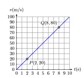
fig 3.3.4.png — Figure $\PageIndex{4}$: Pick two points to compute the slope.

Now, as we move from point $P(2,20)$ to point $Q(8,80)$, the speed changes from $20\mathrm{m} / \mathrm{s}$ to $80\mathrm{m} / \mathrm{s}$. Thus, the change in the speed is:

$\begin{aligned} \Delta v &=80 \mathrm{m} / \mathrm{s}-20 \mathrm{m} / \mathrm{s} \\ &=60 \mathrm{m} / \mathrm{s} \end{aligned}$

Similarly, as we move from point P(2,20) to point Q(8,80), the time changes from 2 seconds to 8 seconds. Thus, the change in time is:

$\begin{aligned} \Delta t &=8 \mathrm{s}-2 \mathrm{s} \\ &=6 \mathrm{s} \end{aligned}$

Now that we have both the change in the dependent and independent variables, we can calculate the slope.

$\begin{aligned} \text { Slope } &=\frac{\Delta v}{\Delta t} \\ &=\frac{60 \mathrm{m} / \mathrm{s}}{6 \mathrm{s}} \\ &=10 \frac{\mathrm{m} / \mathrm{s}}{\mathrm{s}} \end{aligned}$

Therefore, the slope of the line is $10$ meters per second per second ($10(\mathrm{m} / \mathrm{s}) / \mathrm{s}$ or $10\mathrm{m} / \mathrm{s}^{2}$).

The slope of a line does not depend upon the points you select. Let’s try the slope calculation again, using two different points and a more compact presentation of the required calculations. Pick points $P(3,30)$ and $Q(7,70)$ as shown in Figure $\PageIndex{5}$. Using these two new points, the slope is the rate at which the dependent variable $v$ changes with respect to the independent variable $t$.

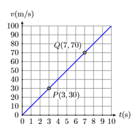
fig 3.3.5.png — Figure $\PageIndex{5}$: The slope does not depend on the points we select on the line.

$\begin{aligned} \text { Slope } &=\frac{\Delta v}{\Delta t} \\ &=\frac{70 \mathrm{m} / \mathrm{s}-30 \mathrm{m} / \mathrm{s}}{7 \mathrm{s}-3 \mathrm{s}} \\ &=\frac{40 \mathrm{m} / \mathrm{s}}{4 \mathrm{s}} \\ &=10 \frac{\mathrm{m} / \mathrm{s}}{\mathrm{s}} \end{aligned}$

Again, the slope of the line is $10(\mathrm{m} / \mathrm{s}) / \mathrm{s}$.

Exercise $\PageIndex{2}$

Starting from rest, an automobile picks up speed at a constant rate of 5 miles per hour every second (5(mi/hr)/s). The constant rate forces the graph of the speed of the object versus time to be a line. Calculate the slope of this line.

Answer: $5(\mathrm{mi} / \mathrm{hr}) / \mathrm{s}$

Example $\PageIndex{2}$ points out the following fact.

Slope is independent of the selected points

It does not matter which two points you pick on the line to calculate its slope.

The next example demonstrates that the slope is also independent of the order of subtraction.

Example $\PageIndex{3}$

Compute the slope of the line passing through the points $P(−1,−2)$ and $Q(3,3)$.

Solution

First, sketch the line passing through the points P(−1,−2) and Q(3,3) (see Figure $\PageIndex{6}$).

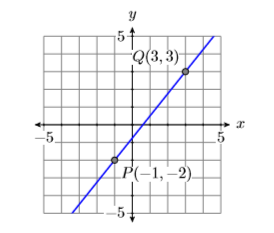
fig 3.3.6.png — Figure $\PageIndex{6}$: Computing the slope of the line passing through the points $P(−1,−2)$ and $Q(3,3)$.

To calculate the slope of the line through the points $P(−1,−2)$ and $Q(3,3)$, we must calculate the change in both the independent and dependent variables. We’ll do this in two different ways.

Warning!

If you are not consistent in the direction you subtract, you will not get the correct answer for the slope.

For example: \[\dfrac{3-(-2)}{-1-3}=-\dfrac{5}{4} \nonumber \]

In this case, we subtracted the $y$-coordinate of point $P(−1,−2)$ from the $y$-coordinate of point $Q(3,3)$, but then we changed horses in midstream, subtracting the $x$-coordinate of point $Q(3,3)$ from the $x$-coordinate of point $P(−1,−2)$. Note that we get the negative of the correct answer.

Method 1

Subtract the coordinates of point $P(−1,−2)$ from the coordinates of point $Q(3,3)$.

\[\begin{aligned} \text { Slope } &=\dfrac{\Delta y}{\Delta x} \\ &=\dfrac{3-(-2)}{3-(-1)} \\ &=\dfrac{5}{4} \end{aligned} \nonumber \]

Method 2

Subtract the coordinates of point $Q(3,3)$ from the coordinates of point $P(−1,−2)$.

\[\begin{aligned} \text { Slope } &=\dfrac{\Delta y}{\Delta x} \\ &=\dfrac{-2-3}{-1-3} \\ &=\dfrac{-5}{-4} \\ &=\dfrac{5}{4} \end{aligned} \nonumber \]

Note that regardless of the direction of subtraction, the slope is $5/4$.

Exercise $\PageIndex{3}$

Compute the slope of the line passing through the points P(−3,1) and Q(2,4).

Answer: $3/5$

Example $\PageIndex{3}$ demonstrates the following fact.

The direction of subtraction does not matter

When calculating the slope of a line through two points $P$ and $Q$, it does not matter which way you subtract, provided you remain consistent in your choice of direction.

The Steepness of a Line

We need to examine whether our definition of slope matches certain expectations.

Slope and steepness of a line

The slope of a line is a number that tells us how steep the line is.

If slope is a number that measures the steepness of a line, then one would expect that a steeper line would have a larger slope.

Example $\PageIndex{4}$

Graph two lines, the first passing through the points $P(−3,−2)$ and $Q(3,2)$ and the second through the points $R(−1,−3)$ and $S(1,3)$. Calculate the slope of each line and compare the results.

Solution

The graphs of the two lines through the given points are shown, the first in Figure $\PageIndex{7}$ and the second in Figure $\PageIndex{8}$. Note that the line in Figure $\PageIndex{7}$ is less steep than the line in Figure $\PageIndex{8}$.

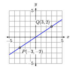
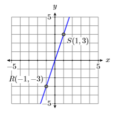
fig 3.3.7.png — Figure $\PageIndex{7}$: This line is less steep than the line on the right. **Figure $\PageIndex{8}$:** This line is steeper than the line on the left.

fig 3.3.8.png — Figure $\PageIndex{7}$: This line is less steep than the line on the right. **Figure $\PageIndex{8}$:** This line is steeper than the line on the left.

Remember, the slope of the line is the rate at which the dependent variable is changing with respect to the independent variable. In both Figure $\PageIndex{7}$ and Figure $\PageIndex{8}$, the dependent variable is $y$ and the independent variable is $x$.

Subtract the coordinates of point $P(−3,−2)$ from the coordinates of point $Q(3,2)$.

\[\begin{aligned} \text { Slope of first line } &=\dfrac{\Delta y}{\Delta x} \\ &=\dfrac{2-(-2)}{3-(-3)} \\ &=\dfrac{4}{6} \\ &=\dfrac{2}{3} \end{aligned} \nonumber \]

Subtract the coordinates of the point $R(−1,−3)$ from the point $S(1,3)$.

\[\begin{aligned} \text { Slope of second line } &=\dfrac{\Delta y}{\Delta x} \\ &=\dfrac{3-(-3)}{1-(-1)} \\ &=\dfrac{6}{2} \\ &=3 \end{aligned} \nonumber \]

Note that both lines go uphill and both have positive slopes. Also, note that the slope of the second line is greater than the slope of the first line. This is consistent with the fact that the second line is steeper than the first.

Exercise $\PageIndex{4}$

Compute the slope of the line passing through the points $P(−2,−3)$ and $Q(2,5)$. Then compute the slope of the line passing through the points $R(−2,−1)$ and $S(5,3)$, and compare the two slopes. Which line is steeper?

Answer: The first line has slope $2$, and the second line has slope $4/7$. The first line is steeper.

In Example $\PageIndex{4}$, both lines slanted uphill and both had positive slopes, the steeper of the two lines having the larger slope. Let’s now look at two lines that slant downhill.

Example $\PageIndex{5}$

Graph two lines, the first passing through the points $P(−3,1)$ and $Q(3,−1)$ and the second through the points $R(−2,4)$ and $S(2,−4)$. Calculate the slope of each line and compare the results.

Solution

The graphs of the two lines through the given points are shown, the first in Figure $\PageIndex{9}$ and the second in Figure $\PageIndex{10}$. Note that the line in Figure $\PageIndex{9}$ goes downhill less quickly than the line in Figure $\PageIndex{10}$. Remember, the slope of the line is the rate at which the dependent variable is changing with respect to the independent variable. In both Figure $\PageIndex{9}$ and Figure $\PageIndex{10}$, the dependent variable is $y$ and the independent variable is $x$.

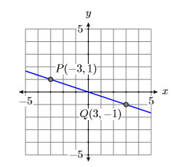
fig 3.3.9.png — Figure $\PageIndex{9}$: This line goes downhill more slowly than the line on the right.

fig3.3.10.png — Figure $\PageIndex{10}$: This line goes downhill more quickly than the line on the left.

Subtract the coordinates of point $P(−3,1)$ from the coordinates of point $Q(3,−1)$.

\[\begin{aligned} \text { Slope of first line } &=\dfrac{\Delta y}{\Delta x} \\ &=\dfrac{-1-1}{3-(-3)} \\ &=\dfrac{-2}{6} \\ &=-\dfrac{1}{3} \end{aligned} \nonumber \]

Subtract the coordinates of point $R(−2,4)$ from the coordinates of point $S(2,−4)$.

\[\begin{aligned} \text { Slope of second line } &=\dfrac{\Delta y}{\Delta x} \\ &=\dfrac{-4-4}{2-(-2)} \\ &=\dfrac{-8}{4} \\ &=-2 \end{aligned} \nonumber \]

Note that both lines go downhill and both have negative slopes. Also, note that the magnitude (absolute value) of the slope of the second line is greater than the magnitude of the slope of the first line. This is consistent with the fact that the second line moves downhill more quickly than the first.

Exercise $\PageIndex{5}$

Compute the slope of the line passing through the points $P(−3,3)$ and $Q(3,−5)$. Then compute the slope of the line passing through the points $R(−4,1)$ and $S(4,−3)$, and compare the two slopes. Which line is steeper?

Answer: The first line has slope $−4/3$, and the second line has slope $−1/2$. The first line is steeper.

What about the slopes of vertical and horizontal lines?

Example $\PageIndex{6}$

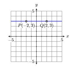
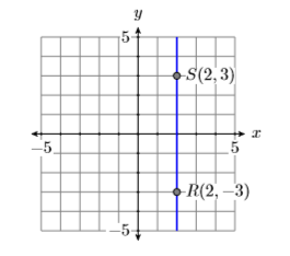
Calculate the slopes of the vertical and horizontal lines passing through the point $(2,3)$.

Solution

First draw a sketch of the vertical and horizontal lines passing through the point (2,3). Next, select a second point on each line as shown in Figures $\PageIndex{11}$ and $\PageIndex{12}$.

fig 3.3.11.png — Figure $\PageIndex{11}$: A horizontal line through $(2,3)$.

fig 3.3.12.png — Figure $\PageIndex{12}$: A vertical line through $(2,3)$.

The slopes of the horizontal and vertical lines are calculated as follows.

Subtract the coordinates of the point $P(−2,3)$ from the coordinates of the point $Q(2,3)$.

\[\begin{aligned} \text { Slope of horizontal line } &=\dfrac{\Delta y}{\Delta x} \\ &=\dfrac{3-3}{2-(-2)} \\ &=\dfrac{0}{4} \\ &=0 \end{aligned} \nonumber \]

Thus, the slope of the horizontal line is zero, which makes sense because a horizontal line neither goes uphill nor downhill.

Subtract the coordinates of the point $(2,−3)$ from the coordinates of the point $S(2,3)$.

\[\begin{aligned} \text { Slope of vertical line } &=\dfrac{\Delta y}{\Delta x} \\ &=\dfrac{3-(-3)}{2-2} \\ &=\dfrac{6}{0} \\ &=\text { undefined } \end{aligned} \nonumber \]

Division by zero is undefined. Hence, the slope of a vertical line is undefined. Again, this makes sense because as uphill lines get steeper and steeper, their slopes increase without bound.

Exercise $\PageIndex{6}$

Calculate the slopes of the vertical and horizontal lines passing through the point $(−4,1)$.

Answer: The slope of the vertical line is undefined. The slope of the second line is $0$.

The Geometry of the Slope of a Line

We begin our geometrical discussion of the slope of a line with an example, calculating the slope of a line passing through the points $P(2,3)$ and $Q(8,8)$. Before we begin we’ll first calculate the change in $y$ and the change in $x$ by subtracting the coordinates of point $P(2,3)$ from the coordinates of point $Q(8,8)$.

\[\begin{aligned} \mathrm{Slope} &=\dfrac{\Delta y}{\dfrac{\Delta x}{\Delta x}} \\ &=\dfrac{8-3}{8-2} \\ &=\dfrac{5}{6} \end{aligned} \nonumber \]

Thus, the slope of the line through the points $P(2,3)$ and $Q(8,8)$ is $5/6$.

To use a geometric approach to finding the slope of the line, first draw the line through the points $P(2,3)$ and $Q(8,8)$ (see Figure $\PageIndex{13}$). Next, draw a right triangle with sides parallel to the horizontal and vertical axes, using the points $P(2,3)$ and $Q(8,8)$ as vertices. As you move from point $P$ to point $R$ in Figure $\PageIndex{13}$, note that the change in $x$ is $\Delta x=6$ (count the tick marks¹).

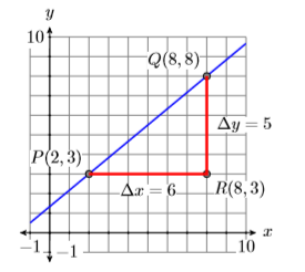
fig 3.3.13.png — Figure $\PageIndex{13}$: Determining the slope of the line from the graph.

As you then move from point $R$ to point $Q$, the change in $y$ is $\Delta y=5$ (count the tick marks). Thus, the slope is $\Delta y / \Delta x=5 / 6$, precisely what we got in the previous computation.

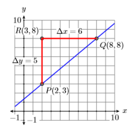
fig 3.3.14.png — Figure $\PageIndex{14}$: Determining the slope of the line from the graph.

For contrast, in Figure $\PageIndex{14}$, we started at the point $P(2,3)$, then moved upward $5$ units and right $6$ units. However, the change in $y$ is still $\Delta y=5$ and the change in $x$ is still $\Delta x=6$ as we move from point $P(2,3)$ to point $Q(8,8)$. Hence, the slope is still $\Delta y / \Delta x=5 / 6$.

Rise over run

In Figure $\PageIndex{14}$, we start at the point $P(2,3)$, then “rise” $5$ units, then “run” $6$ units to the right. For this reason, some like to think of the slope as “rise over run.”

Consider a second example shown in Figure $\PageIndex{15}$. Note that the line slants downhill, so we expect the slope to be a negative number.

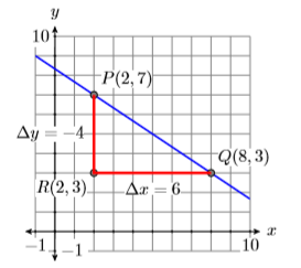
fig 3.3.15.png — Figure $\PageIndex{15}$: Determining the slope of the line from the graph.

In Figure $\PageIndex{15}$, we’ve drawn a right triangle with sides parallel to the horizontal and vertical axes, using the points $P(2,7)$ and $Q(8,3)$ as vertices. As you move from point $P$ to point $R$ in Figure $\PageIndex{15}$, the change in $y$ is $\Delta y=-4$ (count the tick marks and note that your values of y are decreasing as you move from $P$ to $R$). As you move from point $R$ to point $Q$, the change is $x$ is $\Delta x=6$ (count the tick marks and note that your values of $x$ are increasing as you move from $R$ to $Q$). In this case, the “rise” is negative, while the “run” is positive.

Thus, the slope is $\Delta y / \Delta x=-4 / 6$, or $−2/3$. Note that the slope is negative, as anticipated.

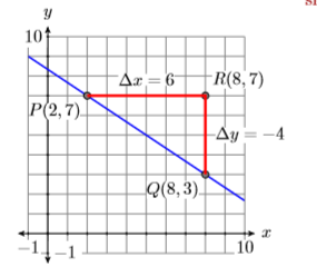
fig 3.3.16.png — Figure $\PageIndex{16}$: Determining the slope of the line from the graph.

In Figure $\PageIndex{16}$, we’ve drawn our triangle on the opposite side of the line. In this case, as you move from point $P$ to point $R$ in Figure $\PageIndex{16}$, the change in $x$ is $\Delta x=6$ (count the tick marks and note that your values of $x$ are increasing as you move from $P$ to $R$). As you move from point $R$ to point $Q$, the change is $y$ is $\Delta y=-4$ (count the tick marks and note that your values of $y$ are decreasing as you move from $R$ to $Q$). Thus, the slope is still $\Delta y / \Delta x=-4 / 6$, or $−2/3$.

We can verify our geometrical calculations of the slope by subtracting the coordinates of the point $P(2,7)$ from the point $Q(8,3)$.
\[\begin{aligned} \text { Slope } &=\dfrac{\Delta y}{\Delta x} \\ &=\dfrac{3-7}{8-2} \\ &=\dfrac{-4}{6} \\ &=-\dfrac{2}{3} \end{aligned} \nonumber \]

This agrees with the calculations made in Figures $\PageIndex{15}$ and $\PageIndex{16}$.

Let’s look at a final example.

Example $\PageIndex{7}$

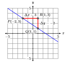
Sketch the line passing through the point $(−2,3)$ with slope $−2/3$.

Solution

The slope is $−2/3$, so the line must go downhill. In Figure $\PageIndex{17}$, we start at the point $P(−2,3)$, move right $3$ units to the point $R(1,3)$, then move down $2$ units to the point $Q(1,1)$. Draw the line through the points $P$ and $Q$ and you are done.

fig 3.3.17.png — Figure $\PageIndex{17}$: Start at $P(−2,3)$, then move right $3$ and down $2$. The resulting line has slope $−2/3$.

In Figure $\PageIndex{18}$, we take a different approach that results in the same line. Start at the point $P(−2,3)$, move downward $4$ units to the point $R(−2,−1)$, then right $6$ units to the point $Q(4,−1)$. Draw a line through the points $P$ and $Q$ and you are done.

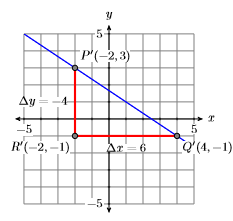
fig 3.3.18.png — Figure $\PageIndex{18}$: Starting at $P(−2,3)$ and moving down $4$ and right $6$ also yields a slope of $−2/3$.

The triangle $PQR$ in Figure $\PageIndex{17}$ is similar to the triangle $PQR$ in Figure $\PageIndex{18}$, so their sides are proportional. Consequently, the slope of the line through points $P(−2,3)$ and $Q(4,−1)$,

\[\begin{aligned} \text { Slope } &=\dfrac{\Delta y}{\Delta x} \\ &=\dfrac{-4}{6} \\ &=-\dfrac{2}{3} \end{aligned} \nonumber \]

reduces to the slope of the line through the points $P$ and $Q$ in Figure $\PageIndex{17}$.

Exercise $\PageIndex{7}$

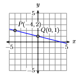
Sketch the line passing through the point $(−4,2)$ with slope $−1/4$.

Answer: $Exercise 3.3.7.png$

A summary of facts about the slope of a line

We present a summary of facts learned in this section.

The slope of a line is the rate at which the dependent variable is changing with respect to the independent variable. If $y$ is the dependent variable and $x$ is the independent variable, then the slope is \[\text {Slope}=\dfrac{\Delta y}{\Delta x} \nonumber \]where $\Delta y$ is the change in $y$ (difference in $y$) and $\Delta x$ is the change in $x$ (difference in $x$).
If a line has positive slope, then the line slants uphill as you “sweep your eyes from left to right.” If two lines have positive slope, then the line with the larger slope rises more quickly.
If a line has negative slope, then the line slants downhill as you “sweep your eyes from left to right.” If two lines have negative slope, then the line having the slope with the larger magnitude falls more quickly.
Horizontal lines have slope zero.
Vertical lines have undefined slope.

References

¹When counting tick marks, make sure you know the amount each tick mark represents. For example, if each tick mark represents two units, and you count six tick marks when evaluating the change in $x$, then $\Delta x=12$.

Search

Text Color

Text Size

Margin Size

Font Type