4.1: Solving Systems by Graphing

In this section we introduce a graphical technique for solving systems of two linear equations in two unknowns. As we saw in the previous chapter, if a point satisfies an equation, then that point lies on the graph of the equation. If we are looking for a point that satisfies two equations, then we are looking for a point that lies on the graphs of both equations; that is, we are looking for a point of intersection.

For example, consider the the two equations:

\[\begin{aligned} x-3 y &=-9 \\ 2 x+3 y &=18 \end{aligned} \nonumber \]

which is called a system of linear equations. The equations are linear equations because their graphs are lines, as shown in Figure \(\PageIndex{1}\). Note that the two lines in Figure \(\PageIndex{1}\) intersect at the point \((3,4)\). Therefore, the point \((3,4)\) should satisfy both equations. Let’s check.

Figure \(\PageIndex{1}\): The point of intersection is a solution of the system of linear equations.

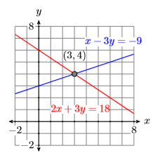
Substitute \(3\) for \(x\) and \(4\) for \(y\).

\[\begin{aligned} x-3 y &=-9 \\ 3-3(4) &=-9 \\ 3-12 &=-9 \\-9 &=-9 \end{aligned} \nonumber \]

Substitute \(3\) for \(x\) and \(4\) for \(y\).

\[\begin{aligned} 2 x+3 y &=18 \\ 2(3)+3(4) &=18 \\ 6+12 &=18 \\ 18 &=18 \end{aligned} \nonumber \]

Hence, the point \((3,4)\) satisfies both equations and is called a solution of the system.

Solution of a linear system

A point \((x,y)\) is called a solution of a system of two linear equations if and only if it satisfied both equations. Furthermore, because a point satisfies an equation if and only if it lies on the graph of the equation, to solve a system of linear equations graphically, we need to determine the point of intersection of the two lines having the given equations.

Let’s try an example.

Example \(\PageIndex{1}\)

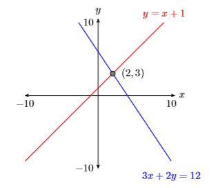
Solve the following system of equations: \[3x+2y =12 \\ y =x+1 \label{system1}\]

Solution

We are looking for the point \((x,y)\) that satisfies both equations; that is, we are looking for the point that lies on the graph of both equations. Therefore, the logical approach is to plot the graphs of both lines, then identify the point of intersection.

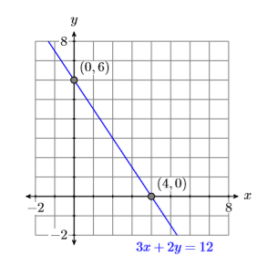
First, let’s determine the \(x\)- and \(y\)-intercepts of \(3x +2y = 12\).

To find the \(x\)-intercept, let \(y = 0\).

\[\begin{aligned} 3 x+2 y &=12 \\ 3 x+2(0) &=12 \\ 3 x &=12 \\ x &=4 \end{aligned} \nonumber \]

To find the \(y\)-intercept, let \(x = 0\).

\[\begin{aligned} 3 x+2 y &=12 \\ 3(0)+2 y &=12 \\ 2 y &=12 \\ y &=6 \end{aligned} \nonumber \]

Hence, the \(x\)-intercept is \((4,0)\) and the \(y\)-intercept is \((0,6)\). These intercepts are plotted in Figure \(\PageIndex{2}\) and the line \(3x +2y = 12\) is drawn through them.

Figure \(\PageIndex{2}\): Drawing the graph of \(3x +2y = 12\).

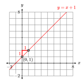
Comparing the second equation \(y = x + 1\) with the slope-intercept form \(y = mx + b\), we see that the slope is \(m = 1\) and they-intercept is \((0,1)\). Plot the intercept \((0,1)\), then go up \(1\) unit and right \(1\) unit, then draw the line (see Figure \(\PageIndex{3}\)).

Figure \(\PageIndex{3}\): Drawing the graph of \(y = x + 1\).

We are trying to find the point that lies on both lines, so we plot both lines on the same coordinate system, labeling each with its equation (see Figure \(\PageIndex{4}\)). It appears that the lines intersect at the point \((2,3)\), making \((x,y) = (2 ,3)\) the solution of System in Example \(\PageIndex{1}\) (see Figure \(\PageIndex{4}\)).

Check: To show that \((x,y) = (2 ,3)\) is a solution of System \ref{system1}, we must show that we get true statements when we substitute \(2\) for \(x\) and \(3\) for \(y\) in both equations of System \ref{system1}.

Figure \(\PageIndex{4}\): The coordinates of the point of intersection is the solution of System \ref{system1}.

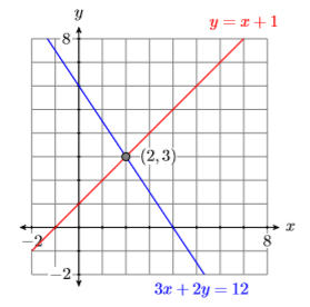
Substituting \(2\) for \(x\) and \(3\) for \(y\) in \(3x +2y = 12\), we get:

\[\begin{aligned} 3 x+2 y &=12 \\ 3(2)+2(3) &=12 \\ 6+6 &=12 \\ 12 &=12 \end{aligned} \nonumber \]

Hence, \((2,3)\) satisfies the equation \(3x +2y = 12\).

Substituting \(2\) for \(x\) and \(3\) for \(y\) in \(y = x + 1\), we get:

\[\begin{array}{l}{y=x+1} \\ {3=2+1} \\ {3=3}\end{array} \nonumber \]

Hence, \((2,3)\) satisfies the equation \(y = x + 1\).

Because \((2,3)\) satisfies both equations, this makes \((2,3)\) a solution of System \ref{system1}.

Exercise \(\PageIndex{1}\)

Solve the following system of equations:

\[\begin{aligned} 2 x-5 y &=-10 \\ y &=x-1 \end{aligned} \nonumber \]

Answer

\((5,4)\)

Example \(\PageIndex{2}\)

Solve the following system of equations: \[3x-5y =-15 \\ 2x+y =-4 \label{system2}\]

Solution

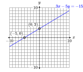
Once again, we are looking for the point that satisfies both equations of the System \ref{system2}. Thus, we need to find the point that lies on the graphs of both lines represented by the equations of System \ref{system2}. The approach will be to graph both lines, then approximate the coordinates of the point of intersection. First, let’s determine the \(x\)- and \(y\)-intercepts of \(3x−5y = −15\).

To find the \(x\)-intercept, let \(y = 0\).

\[\begin{aligned} 3 x-5 y &=-15 \\ 3 x-5(0) &=-15 \\ 3 x &=-15 \\ x &=-5 \end{aligned} \nonumber \]

To find the \(y\)-intercept, let \(x=0\).

\[\begin{aligned} 3 x-5 y &=-15 \\ 3(0)-5 y &=-15 \\-5 y &=-15 \\ y &=3 \end{aligned} \nonumber \]

Hence, the \(x\)-intercept is \((−5,0)\) and the \(y\)-intercept is \((0,3)\). These intercepts are plotted in Figure \(\PageIndex{5}\) and the line \(3x−5y = −15\) is drawn through them.

Figure \(\PageIndex{5}\): Drawing the graph of the line \(3x−5y =−15\).

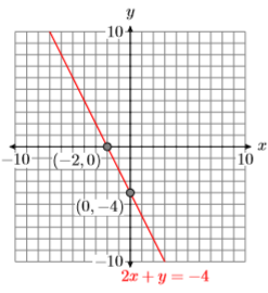
Next, let’s determine the intercepts of the second equation \(2x + y = −4\).

To find the \(x\)-intercept, let \(y = 0\).

\[\begin{aligned} 2 x+y &=-4 \\ 2 x+0 &=-4 \\ 2 x &=-4 \\ x &=-2 \end{aligned} \nonumber \]

To find the \(y\)-intercept, let \(x = 0\).

\[ \begin{aligned} 2 x+y &=-4 \\ 2(0)+y &=-4 \\ y &=-4 \end{aligned} \nonumber \]

Hence, the \(x\)-intercept is \((−2,0)\) and the \(y\)-intercept is \((0,−4)\). These intercepts are plotted in Figure \(\PageIndex{6}\) and the line \(2x + y =−4\) is drawn through them.

Figure \(\PageIndex{6}\): Drawing the graph of the line \(2x + y = −4\).

To find the solution of System \ref{system2}, we need to plot both lines on the same coordinate system and determine the coordinates of the point of intersection. Unlike Example \(\PageIndex{1}\), in this case we’ll have to be content with an approximation of these coordinates. It appears that the coordinates of the point of intersection are approximately \((−2.6,1.4)\) (see Figure \(\PageIndex{7}\)).

Check: Because we only have an approximation of the solution of the system, we cannot expect the solution to check exactly in each equation. However, we do hope that the solution checks approximately.

Figure \(\PageIndex{7}\): The approximate coordinates of the point of intersection are \((−2.6,1.4)\).

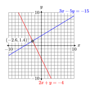
Substitute \((x,y)=(−2.6,1.4)\) into the first equation of System \ref{system2}.

\[\begin{aligned} 3 x-5 y &=-15 \\ 3(-2.6)-5(1.4) &=-15 \\-7.8-7 &=-15 \\-14.8 &=-15 \end{aligned} \nonumber \]

Note that \((x,y)=(−2.6,1.4)\) does not check exactly, but it is pretty close to being a true statement.

Substitute \((x,y)=(−2.6,1.4)\) into the second equation of System \ref{system2}.

\[\begin{aligned} 2 x+y=-4 \\ 2(-2.6)+1.4=-4 \\-5.2+1.4=-4 \\-3.8=-4 \end{aligned} \nonumber \]

Again, note that \((x,y)= (−2.6,1.4)\) does not check exactly, but it is pretty close to being a true statement.

Note

Later in this section we will learn how to use the intersect utility on the graphing calculator to obtain a much more accurate approximation of the actual solution. Then, in Section 4.2 and Section 4.3, we’ll show how to find the exact solution.

Exercise \(\PageIndex{2}\)

Solve the following system of equations:

\[\begin{aligned}-4 x-3 y &=12 \\ x-2 y &=-2 \end{aligned} \nonumber\]

Answer

\((−2.7,−0.4)\)

Exceptional Cases

Most of the time, given the graphs of two lines, they will intersect in exactly one point. But there are two exceptions to this general scenario.

Example \(\PageIndex{3}\)

Solve the following system of equations: \[2x+3y=6\\2x+3y=-6 \label{system3}\]

Solution

Let’s place each equation in slope-intercept form by solving each equation for \(y\).

Solve \(2x +3y = 6\) for \(y\):

\[\begin{aligned} 2 x+3 y &=6 \\ 2 x+3 y-2 x &=6-2 x \\ 3 y &=6-2 x \\ \dfrac{3 y}{3} &=\dfrac{6-2 x}{3} \\ y &=-\dfrac{2}{3} x+2 \end{aligned} \nonumber \]

Solve \(2x +3y =−6\) for \(y\):

\[\begin{aligned} 2 x+3 y &=-6 \\ 2 x+3 y-2 x &=-6-2 x \\ 3 y &=-6-2 x \\ \dfrac{3 y}{3} &=\dfrac{-6-2 x}{3} \\ y &=-\dfrac{2}{3} x-2 \end{aligned} \nonumber \]

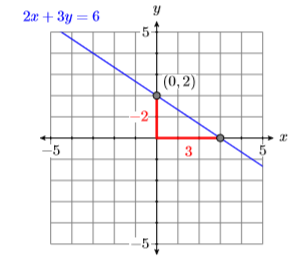
Comparing \(y =(−2/3)x+2\) with the slope-intercept form \(y = mx+b\) tells us that the slope is \(m = −2/3\) and they-intercept is \((0,2)\). Plot the intercept \((0,2)\), then go down \(2\) units and right \(3\) units and draw the line (see Figure \(\PageIndex{8}\)).

Figure \(\PageIndex{8}\): Drawing the graph of the line \(2x +3y = 6\).

Comparing \(y =( −2/3)x − 2\) with the slope-intercept form \(y = mx + b\) tells us that the slope is \(m = −2/3\) and they-intercept is \((0,−2)\). Plot the intercept \((0 ,−2)\), then go down \(2\) units and right \(3\) units and draw the line (see Figure \(\PageIndex{9}\)).

Figure \(\PageIndex{9}\): Drawing the graph of the line \(2x +3y =−6\).

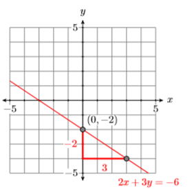
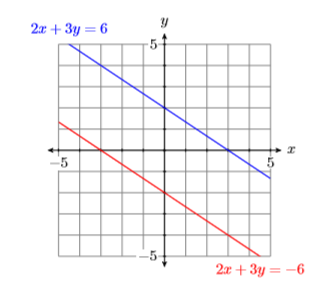
To find the solution of System \ref{system3}, draw both lines on the same coordinate system (see Figure \(\PageIndex{10}\)). Note how the lines appear to be parallel (they don’t intersect). The fact that both lines have the same slope \(−2/3\) confirms our suspicion that the lines are parallel. However, note that the lines have different \(y\)-intercepts. Hence, we are looking at two parallel but distinct lines (see Figure \(\PageIndex{10}\)) that do not intersect. Hence, System \ref{system3} has no solution.

Figure \(\PageIndex{10}\): The lines \(2x+3y = 6\) and \(2x+3y = −6\) are parallel, distinct lines.

Exercise \(\PageIndex{3}\)

Solve the following system of equations:

\[\begin{aligned} x-y &=3 \\-2 x+2 y &=4 \end{aligned} \nonumber \]

Answer

No solution.

Example \(\PageIndex{4}\)

Solve the following system of equations: \[x-y=3 \\-2 x+2 y=-6 \label{system4}\]

Solution

Let’s solve both equations for \(y\).

Solve \(x−y = 3\) for \(y\):

\[\begin{aligned} x-y &=3 \\ x-y-x &=3-x \\-y &=-x+3 \\-1(-y) &=-1(-x+3) \\ y &=x-3 \end{aligned} \nonumber \]

Solve \(−2x +2y =−6\) for \(y\):

\[\begin{aligned}-2 x+2 y &=-6 \\-2 x+2 y+2 x &=-6+2 x \\ 2 y &=2 x-6 \\ \dfrac{2 y}{2} &=\dfrac{2 x-6}{2} \\ y &=x-3 \end{aligned} \nonumber \]

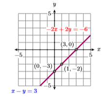
Both lines have slope \(m = 1\), and both have the same \(y\)-intercept \((0,−3)\). Hence, the two lines are identical (see Figure \(\PageIndex{11}\)). Hence, System \ref{system4} has an infinite number of points of intersection. Any point on either line is a solution of the system. Examples of points of intersection (solutions satisfying both equations) are \((0,−3)\), \((1,−2)\), and \((3,0)\).

Figure \(\PageIndex{11}\): \(x − y = 3\) and \(−2x +2y = −6\) are the same line.

Alternate solution:

A much easier approach is to note that if we divide both sides of the second equation \(−2x +2y = −6\) by \(−2\), we get:

\[\begin{aligned} -2x+2y &= -6 \quad {\color {Red} \text { Second equation in System }} \ref{system4}. \\ \dfrac{-2 x+2 y}{-2} &= \dfrac{-6}{-2} \quad \color {Red} \text { Divide both sides by }-2 \\ \dfrac{-2 x}{-2}+\dfrac{2 y}{-2} &= \dfrac{-6}{-2} \quad \color {Red} \text { Distribute }-2 \\ x-y &= 3 \quad \color {Red} \text { Simplify. } \end{aligned} \nonumber \]

Hence, the second equation in System \ref{system4} is identical to the first. Thus, there are an infinite number of solutions. Any point on either line is a solution.

Exercise \(\PageIndex{4}\)

Solve the following system of equations:

\[\begin{aligned}-6 x+3 y &=-12 \\ 2 x-y &=4 \end{aligned} \nonumber \]

Answer

There are an infinite number of solutions. The lines are identical, so any point on either line is a solution.

Examples \(\PageIndex{1}\), \(\PageIndex{2}\), \(\PageIndex{3}\), and \(\PageIndex{4}\) lead us to the following conclusion.

Number of solutions of a linear system

When dealing with a system of two linear equations in two unknowns, there are only three possibilities:

1. There is exactly one solution.
2. There are no solutions.
3. There are an infinite number of solutions.

Solving Systems with the Graphing Calculator

We’ve already had experience graphing equations with the graphing calculator. We’ve also used the TRACE button to estimate points of intersection. However, the graphing calculator has a much more sophisticated tool for finding points of intersection. In the next example we’ll use the graphing calculator to find the solution of System \ref{system1} of Example \(\PageIndex{1}\).

Example \(\PageIndex{5}\)

Use the graphing calculator to solve the following system of equations: \[3x+2y=12 \\ y=x+1 \label{system5} \]

Solution

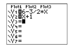
To enter an equation in the Y= menu, the equation must first be solved for \(y\). Hence, we must first solve \(3x +2y = 12\) for \(y\).

\[\begin{aligned} 3x+2y &=12 \quad \color {Red} \text { Original equation. } \\ 2y &= 12-3x \quad \color {Red} \text { Subtract } 3x \text { from both sides of the equation. } \\ \dfrac{2y}{2} &= \dfrac{12-3 x}{2} \quad \color {Red} \text { Divide both sides by } 2 \\ y &= \dfrac{12}{2}-\dfrac{3 x}{2} \quad \color {Red} \text { On the left, simplify. On the right, } \\ y &= 6-\dfrac{3}{2} x \quad \color {Red} \text { Simplify. } \end{aligned}\]

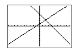
We can now substitute both equations of System \ref{system5} into the Y= menu (see Figure \(\PageIndex{12}\)).

Figure \(\PageIndex{12}\): Enter System \ref{system5} equations into the Y= menu.

Select 6:ZStandard from the ZOOM menu to produce the graphs shown in Figure \(\PageIndex{13}\).

Figure \(\PageIndex{13}\): Select 6:ZStandard to produce the graphs of the System \ref{system5} equations.

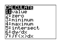
The question now becomes “How do we calculate the coordinates of the point of intersection?” Look on your calculator case just above the TRACE button on the top row of buttons, where you’ll see the word CAlC, painted in the same color as the 2ND key. Press the 2ND key, then the TRACE button, which will open the CALCULATE menu shown in Figure \(\PageIndex{14}\).

Figure \(\PageIndex{14}\): Press 2ND, then TRACE to open the CALCULATE menu. Then select 5:intersect to produce the screen in Figure \(\PageIndex{15}\).

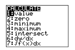
Note

Having the calculator ask “First curve,” “Second curve,” when there are only two curves on the screen may seem annoying. However, imagine the situation when there are three or more curves on the screen. Then these questions make good sense. You can change your selection of “First curve” or “Second curve” by using the up-and-down arrow keys to move the cursor to a different curve.

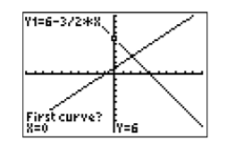
Select 5:intersect. The result is shown in Figure \(\PageIndex{15}\). The calculator has placed the cursor on the curve \(y =6−(3/2)x\) (see upper left corner of your viewing screen), and in the lower left corner the calculator is asking you if you want to use the selected curve as the “First curve.” Answer “yes” by pressing the ENTER button.

Figure \(\PageIndex{15}\): Press the ENTER key on your calculator to say “yes” to the “First curve” selection.

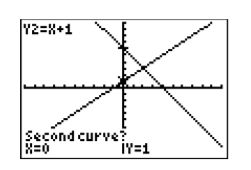
The calculator responds as shown Figure \(\PageIndex{16}\). The cursor jumps to the curve \(y = x + 1\) (see upper left corner of your viewing window), and in the lower left corner the calculator is asking you if you want to use the selected curve as the “Second curve.” Answer “yes” by pressing the ENTER key again.

Figure \(\PageIndex{16}\): Press the ENTER key on your calculator to say “yes” to the “Second curve” selection.

The calculator responds as shown Figure \(\PageIndex{17}\), asking you to “Guess.” In this case, leave the cursor where it is and press the ENTER key again to signal the calculator that you are making a guess at the current position of the cursor.

Figure \(\PageIndex{17}\): Press the ENTER key to signal the calculator that you are satisfied with the current position of the cursor as your guess.

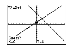
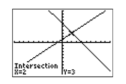
The result of pressing ENTER to the “Guess” question in Figure \(\PageIndex{17}\) is shown in Figure \(\PageIndex{18}\), where the calculator now provides an approximation of the the coordinates of the intersection point on the bottom edge of the viewing window. Note that the calculator has placed the cursor on the point of intersection in Figure \(\PageIndex{17}\) and reports that the approximate coordinates of the point of intersection are \((2,3)\).

Figure \(\PageIndex{18}\): Read the approximate coordinates of the point of intersection along the bottom edge of the viewing window.

Note

In later sections, when we investigate the intersection of two graphs having more than one point of intersection, guessing will become more important. In those future cases, we’ll need to use the left-and-right arrow keys to move the cursor near the point of intersection we wish the calculator to find.

Reporting your solution on your homework. In reporting your solution on your homework paper, follow the Calculator Submission Guidelines from Chapter 3, Section 2. Make an accurate copy of the image shown in your viewing window. Label your axes \(x\) and \(y\). At the end of each axis, put the appropriate value of \(\mathrm{Xmin}, \mathrm{Xmax}, \mathrm{Ymin}\), and \(\mathrm{Ymax}\) reported in your calculator’s WINDOW menu. Use a ruler to draw the lines and label each with their equations. Finally, label the point of intersection with its coordinates (see Figure \(\PageIndex{19}\)). Unless instructed otherwise, always report every single digit displayed on your calculator.

Figure \(\PageIndex{19}\): Reporting your result on your homework paper.

Exercise \(\PageIndex{5}\)

Solve the following system of equations:

\[\begin{aligned} 2 x-5 y &=9 \\ y &=2 x-5 \end{aligned} \nonumber \]

Answer

\((2,-1)\)

Sometimes you will need to adjust the parameters in the WINDOW menu so that the point of intersection is visible in the viewing window.

Example \(\PageIndex{6}\)

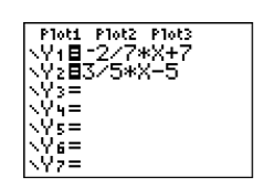
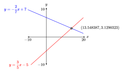
Use the graphing calculator to find an approximate solution of the following system: \[y=-\dfrac{2}{7} x+7\\ y=\dfrac{3}{5} x-5 \label{system6} \]

Solution

Each equation of System \ref{system6} is already solved for \(y\), so we can proceed directly and enter them in the Y= menu, as shown in Figure \(\PageIndex{20}\). Select 6:ZStandard from the ZOOM menu to produce the image shown in Figure \(\PageIndex{21}\).

Figure \(\PageIndex{20}\): Enter the equations of System \ref{system6}.

Figure \(\PageIndex{21}\): Select 6:ZStandard to produce this window.

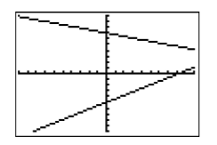
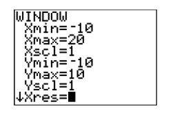
Obviously, the point of intersection is off the screen to the right, so we’ll have to increase the value of \(\mathrm{Xmax}\) (set \(\mathrm{Xmax}=20\)) as shown in Figure \(\PageIndex{22}\). Once you have made that change to \(\mathrm{Xmax}\), press the GRAPH button to produce the image shown in Figure \(\PageIndex{23}\).

Figure \(\PageIndex{22}\): Change \(\mathrm{Xmax}\) to \(20\).

Figure \(\PageIndex{23}\): Press the GRAPH button to produce this window.

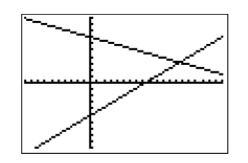
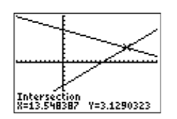
Now that the point of intersection is visible in the viewing window, press 2ND CALC and select 5:intersect from the CALCULATE menu (see Figure \(\PageIndex{24}\)). Make three consecutive presses of the ENTER button to respond to “First curve,” “Second curve,” and “Guess.” The calculator responds with the image in Figure \(\PageIndex{25}\). Thus, the solution of System \ref{system6} is approximately \((x,y) ≈ (13.54837,3.1290323)\).

Figure \(\PageIndex{24}\): Press 2ND CALC to open the CALCULATE menu. Select 5:intersect to find the point of intersection.

Figure \(\PageIndex{25}\): Three consecutive presses of the ENTER key produce the coordinates shown at the bottom of the viewing window.

\(\color {Red}Warning!\)

Your calculator is an approximating machine. It is quite likely that your solutions might differ slightly from the solution presented in Figure \(\PageIndex{25}\) in the last \(2-3\) places.

Reporting your solution on your homework:

In reporting your solution on your homework paper, follow the Calculator Submission Guidelines from Chapter 3, Section 2. Make an accurate copy of the image shown in your viewing window. Label your axes \(x\) and \(y\). At the end of each axis, put the appropriate value of \(\mathrm{Xmin}, \mathrm{Xmax}, \mathrm{Ymin}\), and \(\mathrm{Ymax}\) reported in your calculator’s WINDOW menu. Use a ruler to draw the lines and label each with their equations. Finally, label the point of intersection with its coordinates (see Figure \(\PageIndex{26}\)). Unless instructed otherwise, always report every single digit displayed on your calculator.

Figure \(\PageIndex{26}\): Reporting your result on your homework paper.

Exercise \(\PageIndex{6}\)

Solve the following system of equations:

\[\begin{aligned} y &= \dfrac{3}{2} x+6 \\ y &= -\dfrac{6}{7} x-4\end{aligned} \nonumber \]

Answer

\((-4.2,-0.4)\)