4.3: Solving Systems by Elimination
- Page ID
- 19872
When both equations of a system are in standard form \(Ax + By = C\), then a process called elimination is usually the best procedure to use to find the solution of the system. Elimination is based on two simple ideas, the first of which should be familiar.
- Multiplying both sides of an equation by a non-zero number does not change its solutions. Thus, the equation \[x+3 y=7 \label{Eq4.3.1}\]will have the same solutions (it’s the same line) as the equation obtained by multiplying Equation \ref{Eq4.3.1} by \(2\): \[2 x+6 y=14 \]
- Adding two true equations produces another true equation. For example, consider what happens when you add \(4 = 4\) to \(5 = 5\).\[\begin{aligned} 4 &=4 \\ 5 &=5 \\ \hline 9 &=9 \end{aligned} \nonumber\]
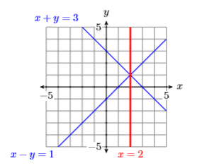
Even more importantly, consider what happens when you add two equations that have \((2,1)\) as a solution. The result is a third equation whose graph also passes through the solution.
\[\begin{array}{rlrl}{x+y} & {=} & {3} \\ {x-y} & {=} & {1} \\ \hline 2 x\;\;\;\;\; & {=} & {4} \\ {x} \;\;\;\;\;& {=} & {2}\end{array} \nonumber \]
fact
Adding a multiple of an equation to a second equation produces an equation that passes through the same solution as the first two equations.
One more important thing to notice is the fact that when we added the equations \[\begin{aligned} x+y &=3 \\ x-y &=1 \\ \hline 2 x \;\;\;\;\;&=4 \end{aligned} \nonumber \]
the variable \(y\) was eliminated. This is where the elimination method gets its name. The strategy is to somehow add the equations of a system with the intent of eliminating one of the unknown variables. However, sometimes you need to do a little bit more than simply add the equations. Let’s look at an example.
Example \(\PageIndex{1}\)
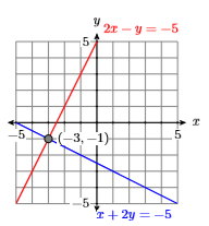
Solve the following system of equations:
\[x+2y=-5 \label{Eq4.3.3} \]
\[2x-y=-5 \label{Eq4.3.4} \]
Solution
Our focus will be on eliminating the variable \(x\). Note that if we multiply Equation \ref{Eq4.3.3} by \(−2\), then add the result to Equation \ref{Eq4.3.4}, the \(x\) terms will be eliminated.
\[\begin{aligned}-2 x-4 y &=10 \quad {\color{Red} \text{Multiply equation}} \ref{Eq4.3.3} \color{Red} \text{ by } -2\\ 2 x-y &=-5 \quad {\color{Red} \text{Multiply equation}} \ref{Eq4.3.4}\\ \hline-5 y &=5 \quad \color{Red} \text {Add the equations.} \end{aligned} \nonumber \]
Divide both sides of \(−5y = 5\) by \(−5\) to get \(y =−1\). To find the corresponding value of \(x\), substitute \(−1\) for \(y\) in Equation \ref{Eq4.3.3} (or Equation \ref{Eq4.3.4}) and solve for \(x\).
\[\begin{aligned} x+2y &= -5 \quad {\color{Red} \text { Equation }} \ref{Eq4.3.3} \\ x+2(-1) &= -5 \quad \color{Red} \text { Substitute }-1 \text { for } y \\ x &= -3 \quad \color{Red} \text { Solve for } x . \end{aligned} \nonumber \]
Check: To check, we need to show that the point \((x,y)=( −3,1)\) satisfies both equations.
Substitute \((x,y)=( −3,−1)\) into Equation \ref{Eq4.3.3}.
\[\begin{aligned} x+2 y &=-5 \\-3+2(-1) &=-5 \\-5 &=-5 \end{aligned} \nonumber \]
Substitute \((x,y)=( −3,−1)\) intoEquation \ref{Eq4.3.4}.
\[\begin{aligned} 2 x-y &=-5 \\ 2(-3)-(-1) &=-5 \\-5 &=-5 \end{aligned} \nonumber \]
Thus, the point \((x,y)=(−3,−1)\) satisfies both equations and is therefore the solution of the system.
Exercise \(\PageIndex{1}\)
Solve the following system of equations:
\[\begin{aligned} x+3 y &=14 \\-8 x-3 y &=-28 \end{aligned} \nonumber \]
- Answer
-
\((2,4)\)
To show that you have the option of which variable you choose to eliminate, let’s try Example \(\PageIndex{1}\) a second time, this time eliminating \(y\) instead of \(x\).
Example \(\PageIndex{2}\)
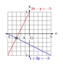
Solve the following system of equations:
\[x+2y=-5 \label{Eq4.3.5} \]
\[2x-y=-5 \label{Eq4.3.6} \]
Solution
This time we focus on eliminating the variable \(y\). We note that if we multiply Equation \ref{Eq4.3.6} by \(2\), then add the result to Equation \ref{Eq4.3.5}, the \(y\) terms will be eliminated.
\[\begin{aligned} x+2y &=-5 \quad {\color {Red} \text {Equation }} \ref{Eq4.3.5}\\ 4 x-2y &=-10 \quad {\color {Red} \text {Multiple equation }} \ref{Eq4.3.6} \color {Red} \text { by } 2\\ \hline 5x \;\;\;\;\;\;\;&=-15 \quad \color {Red} \text {Add the equations.} \end{aligned} \nonumber \]
Divide both sides of \(5x = −15\) by \(5\) to get \(x =−3\). To find the corresponding value of \(y\), substitute \(−3\) for \(x\) in Equation \ref{Eq4.3.5} (or Equation \ref{Eq4.3.6}) and solve for \(y\).
\[\begin{aligned} x+2y &= -5 \quad {\color {Red} \text { Equation }} \ref{Eq4.3.5} \\ -3+2y &= -5 \quad \color {Red} \text { Substitute }-3 \text { for } x \\ 2y &= -2 \quad \color {Red} \text { Add } 3 \text { to both sides. } \\ y &= -1 \quad \color {Red} \text { Divide both sides by } 2 \end{aligned} \nonumber \]
Hence, \((x,y)=(−3,−1)\), just as in Example \(\PageIndex{1}\), is the solution of the system.
Sometimes elimination requires a thought process similar to that of finding a common denominator.
Example \(\PageIndex{3}\)
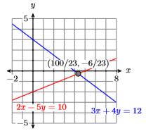
Solve the following system of equations:
\[3x+4y=12 \label{Eq4.3.7} \]
\[2x-5y=10 \label{Eq4.3.8} \]
Solution
Let’s focus on eliminating the \(x\)-terms. Note that if we multiply Equation \ref{Eq4.3.7} by \(2\), then multiply Equation \ref{Eq4.3.8} by \(−3\), the \(x\)-terms will be eliminated when we add the resulting equations.
\[\begin{aligned} 6x+8y &= 24 \quad {\color {Red} \text {Multiple equation }} \ref{Eq4.3.7} \color {Red} \text { by } 2\\ -6x+15y &= -30 \quad {\color {Red} \text {Multiple equation }} \ref{Eq4.3.8} \color {Red} \text { by } 2\\ \hline 23y &= -6 \quad \color {Red} \text {Add the equations.} \end{aligned} \nonumber \]
Hence, \(y = −6/23\).
At this point, we could substitute \(y = −6/23\) in either equation, then solve the result for \(x\). However, working with \(y = −6/23\) is a bit daunting, particularly in the light of elimination being easier. So let’s use elimination again, this time focusing on eliminating \(y\). Note that if we multiply Equation \ref{Eq4.3.7} by \(5\), then multiply Equation \ref{Eq4.3.8} by \(4\), when we add the results, the \(y\)-terms will be eliminated.
\[\begin{aligned} 5x+20y &= 60 \quad {\color {Red} \text {Multiple equation }} \ref{Eq4.3.7} \color {Red} \text { by } 5\\ 8x-20y &= 40 \quad {\color {Red} \text {Multiple equation }} \ref{Eq4.3.8} \color {Red} \text { by } 4\\ \hline 23x\;\;\;\;\;\;\;\;\; &= 100 \quad \color {Red} \text {Add the equations.} \end{aligned} \nonumber \]
Thus, \(x = 100/23\), and the system of the system is \((x,y) = (100/23,−6/23)\).
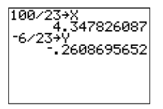
Check: Let’s use the graphing calculator to check the solution. First, store \(100/23\) in \(X\), then \(−6/23\) in \(Y\) (see Figure \(\PageIndex{5}\)). Next, enter the left-hand sides of equations \ref{Eq4.3.7} and \ref{Eq4.3.8}.
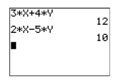
Note that both calculations in Figure \(\PageIndex{6}\) provide the correct right-hand sides for equations \ref{Eq4.3.7} and \ref{Eq4.3.8}. Thus, the solution \((x,y) = (100/23,−6/23)\) checks.
Exercise \(\PageIndex{3}\)
Solve the following system of equations:
\[\begin{aligned}-14 x+9 y &=94 \\ 7 x+3 y &=-62 \end{aligned} \nonumber \]
- Answer
-
\((-8,-2)\)
Exceptional Cases
In the previous section, we saw that if the substitution method led to a false statement, then we have parallel lines. The same thing can happen with the elimination method of this section.
Example \(\PageIndex{4}\)
Solve the following system of equations:
\[x+y=3 \label{Eq4.3.9} \]
\[2x+2y=6 \label{Eq4.3.10} \]
Solution
Let’s focus on eliminating the \(x\)-terms. Note that if we multiply Equation \ref{Eq4.3.9} by \(−2\), the \(x\)-terms will be eliminated when we add the resulting equations.
\[\begin{aligned} -2x-2y &= -6 \quad {\color {Red} \text {Multiple equation }} \ref{Eq4.3.9} \color {Red} \text { by } -2\\ 2x+2y &= -6 \quad {\color {Red} \text {Equation }} \ref{Eq4.3.10} \\ \hline 0 &= -12 \quad \color {Red} \text {Add the equations.} \end{aligned} \nonumber \]
Because of our experience with this solving this exceptional case with substitution, the fact that both variables have disappeared should not be completely surprising. Note that this last statement is false, regardless of the values of \(x\) and \(y\). Hence, the system has no solution.
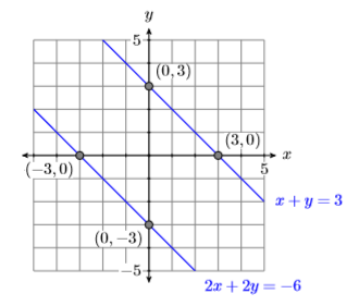
Indeed, if we find the intercepts of each equation and plot them, then we can easily see that the lines of this system are parallel (see Figure \(\PageIndex{7}\)). Parallel lines never intersect, so the system has no solutions.
Exercise \(\PageIndex{4}\)
Solve the following system of equations:
\[\begin{aligned} 5 x-4 y &=-16 \\ 15 x-12 y &=49 \end{aligned} \nonumber \]
- Answer
-
no solution
In the previous section, we saw that if the substitution method led to a true statement, then we have the same lines. The same thing can happen with the elimination method of this section.
Example \(\PageIndex{5}\)
Solve the following system of equations:
\[x-7y=4 \label{Eq4.3.11} \]
\[-3x+21y=-12 \label{Eq4.3.12} \]
Solution
If we are not on automatic pilot late at night doing our homework, we might recognize that the equations \ref{Eq4.3.11} and \ref{Eq4.3.12} are identical. But it’s also conceivable that we don’t see that right away and begin the elimination method. Let’s multiply the first equation by \(3\), then add. This will eliminate the \(x\)-terms.
\[\begin{aligned} 3x-21y &= 12 \quad {\color {Red} \text {Multiple equation }} \ref{Eq4.3.11} \color {Red} \text { by } 3\\ 3x+21y &= -12 \quad {\color {Red} \text {Equation }} \ref{Eq4.3.12} \\ \hline 0 &= 0 \quad \color {Red} \text {Add the equations.} \end{aligned} \nonumber \]
Again, all of the variables have disappeared! However, this time the last statement is true, regardless of the values of \(x\) and \(y\).
Notice that if we multiply Equation \ref{Eq4.3.11} by \(−3\), then we have two identical equations.
\[\begin{aligned} -3x+21y &= -12 \quad {\color {Red} \text {Multiple equation }} \ref{Eq4.3.11} \color {Red} \text { by } 3\\ -3x+21y &= -12 \quad {\color {Red} \text {Equation }} \ref{Eq4.3.12} \end{aligned} \nonumber \]
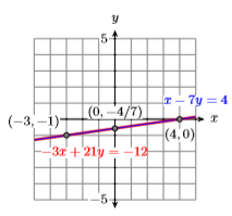
The equations are identical! Hence, there are an infinite number of points of intersection. Indeed, any point on either line is a solution. Example points of solution are \((−3,−1)\), \((0,−4/7)\), and \((4,0)\).
Exercise \(\PageIndex{5}\)
Solve the following system of equations:
\[\begin{array}{c}{2 x-7 y=4} \\ {8 x-28 y=16}\end{array} \nonumber \]
- Answer
-
There are an infinite number of solutions. Examples of solution points are \((2,0)\), \((9,2)\), and \((−5,−2)\).


