5.2: Polynomials

We begin with the definition of a term.

Definition: Term

A term is either a single number (called a constant term) or the product of a number and one or more variables.

For example, each of the following is a term.

\[ -5 \quad-3 x^{2} \quad 12 y^{2} z^{3} \quad 13 a^{2} b c^{3} \nonumber \]

Note how the first term is a single number, while the remaining terms are products of a number and one or more variables. For example, \(−3x^2\) is the product of \(−3\), \(x\), and \(x\).

Definition: Coefficient

When a term is a product of a number and one or more variables, the number is called the coefficient of the term. In the case of a term that is a single number, the number itself is called the coefficient.

Thus, for example, the coefficients of the terms \[-5 \quad-3 x^{2} \quad 12 y^{2} z^{3} \quad 13 a^{2} b c^{3} \nonumber \]are \(−5\), \(−3\), \(12\), and \(13\), respectively.

Definition: Degree

The degree of a term is the sum of the exponents on each variable of the term. A constant term (single number with no variables) has degree zero.

Thus, for example, the degrees of the terms \[-5 \quad-3 x^{2} \quad 12 y^{2} z^{3} \quad 13 a^{2} b c^{3} \nonumber \]are \(0\), \(2\), \(5\), and \(6\), respectively. In the last example, note that \(13a^2bc^3\) is equivalent to \(13a^2b^1c^3\), so adding exponents, we get:

\[\begin{aligned} \text { Degree of } 13 a^{2} b c^{3} &=\text { Degree of } 13 a^{2} b^{1} c^{3} \\ &=2+1+3 \\ &=6 \end{aligned} \nonumber \]

Definition: Monomial

The words monomial and term are equivalent.

Thus, \[-5 \quad-3 x^{2} \quad 12 y^{2} z^{3} \quad 13 a^{2} b c^{3} \nonumber \]are monomials.

Definition: Binomial

A binomial is a mathematical expression containing exactly two terms, separated by plus or minus signs.

For example, each of the mathematical expressions \[2 x+3 y \quad-3 a^{2}-3 b^{2} \quad x y+7 \quad-3 x^{2} y+5 x y^{2} \nonumber \]is a binomial. Each expression has exactly two terms.

Definition: Trinomial

A trinomial is a mathematical expression containing exactly three terms, separated by plus or minus signs.

For example, each of the mathematical expressions \[2 x^{2}+3 x+7 \quad a^{2}+2 a b+b^{2} \quad x^{4}-2 x^{2} y^{2}+3 y^{4} \nonumber \]is a trinomial. Each expression has exactly three terms.

A bicycle has two wheels, a binomial has two terms. A tricycle has three wheels, a trinomial has three terms. But once we get past three terms, the assignment of special names ceases and we use the generic word polynomial, which means “many terms.”

Definition: Polynomial

A polynomial is a many-termed mathematical expression, with terms separated by plus or minus signs. The coefficients of a polynomial are the coefficients of its terms.

Each of the previous expressions, \[12 y^{2} z^{3} \quad-3 a^{2}-3 b^{2} \quad x^{4}-2 x^{2} y^{2}+3 y^{4} \nonumber \]though assigned the particular names monomial, binomial, and trinomial, respectively, are also “many-termed” expressions and can also be called polynomials. However, because the word polynomial means “many terms,” we can also use the word polynomial to describe mathematical expressions with more than three terms, such as: \[x^{4}-4 x^{3} y+6 x^{2} y^{2}-4 x y^{3}+y^{4} \nonumber \]The coefficients of \(x^{4}-4 x^{3} y+6 x^{2} y^{2}-4 x y^{3}+y^{4}\) are \(1\), \(−4\), \(6\), \(−4\), and \(1\).

Ascending and Descending Powers

When asked to simplify a polynomial expression, we should combine any like terms we find, and when possible, arrange the answer in ascending or descending powers.

Example \(\PageIndex{1}\)

Simplify the following polynomial expression, arranging your answer in the descending powers of \(x\). Once you’ve completed that task, make a second arrangement, ordering your terms in ascending powers of \(x\). \[2 x^{3}+7 x-3 x^{2}+11 x+8 x^{2}+11+15 x \nonumber \]

Solution

In order to arrange our answer in descending powers of \(x\), we want to place the term with the highest power of \(x\) first and the term with the lowest power of \(x\) last. We use the commutative and associative properties to change the order and regroup, then we combine like terms.

\[\begin{aligned} 2 x^{3}+7 x &-3 x^{2}+11 x+8 x^{2}+11+15 x \\ &=2 x^{3}+\left(-3 x^{2}+8 x^{2}\right)+(7 x+11 x+15 x)+11 \\ &=2 x^{3}+5 x^{2}+33 x+11 \end{aligned} \nonumber \]

Note how the powers of \(x\) start at \(3\), then go down in order.

To arrange our final answer in ascending powers of \(x\), we put the lowest power of \(x\) first, then the highest power of \(x\) last, regrouping and combining like terms.

\[\begin{aligned} 2 x^{3}+7 x &-3 x^{2}+11 x+8 x^{2}+11+15 x \\ &=11+(7 x+11 x+15 x)+\left(-3 x^{2}+8 x^{2}\right)+2 x^{3} \\ &=11+33 x+5 x^{2}+2 x^{3} \end{aligned} \nonumber \]

Note how we start with the constant term, then the powers of \(x\) increase in order.

Exercise \(\PageIndex{1}\)

Simplify the following polynomial, and arrange your answer in ascending powers of \[3 x^{2}-5 x^{3}+8 x+9 x^{2}-7 x+2 x^{3} \nonumber \]

Answer

\(x+12 x^{2}-3 x^{3}\)

When we have a polynomial in a single variable, such as the polynomial in Example \(\PageIndex{1}\), arranging the terms in ascending or descending order is fairly straightforward. However, a polynomial in two or more variables is a bit more difficult, and sometimes impossible, to arrange in a decent order.

Example \(\PageIndex{2}\)

Simplify the following polynomial expression, then arrange your answer in descending powers of \(x\).\[x^{3}+2 x y^{2}-6 x^{2} y+y^{3}-3 x y^{2}+4 x^{2} y \nonumber \]

Solution

We’ll again use the commutative and associative properties to change the order and regroup, putting the terms with the highest powers of \(x\) first, then follow with terms containing lower powers of \(x\) in order.

\[\begin{aligned} x^{3}+2 x y^{2} &-6 x^{2} y+y^{3}-3 x y^{2}+4 x^{2} y \\ &=x^{3}+\left(-6 x^{2} y+4 x^{2} y\right)+\left(2 x y^{2}-3 x y^{2}\right)+y^{3} \\ &=x^{3}-2 x^{2} y-x y^{2}+y^{3} \end{aligned} \nonumber \]

Note that this is a very natural order, the powers of \(x\) decrease while simultaneously the powers of \(y\) increase.

Exercise \(\PageIndex{2}\)

Simplify the following polynomial, and arrange your answer in descending powers of \(x\): \[-4 x^{2} y^{2}+3 x y^{3}+6 x^{3} y-x y^{3}+2 x^{2} y^{2} \nonumber \]

Answer

\(6 x^{3} y-2 x^{2} y^{2}+2 x y^{3}\)

Not all examples will have nice ordering presented in Example \(\PageIndex{2}\), with the powers of one variable descending while the powers of the other variable simultaneously ascends. Sometimes we have to make some very subjective choices on the ordering of terms.

Example \(\PageIndex{3}\)

Simplify the following polynomial expression, then arrange your answer in some sort of reasonable order. \[a^{3} b^{3}+2 a^{2} b-3 a^{2} b^{3}+4 a^{3} b^{3}+5 a^{4}+3 a^{2} b+b^{5} \nonumber \]

Solution

Let’s try to arrange the terms so that the powers of a descend. Again, we use the commutative and associative properties to change the order and regroup.

\[\begin{aligned} a^{3} b^{3}+2 a^{2} b &-3 a^{2} b^{3}+4 a^{3} b^{3}+5 a^{4}+3 a^{2} b+b^{5} \\ &=5 a^{4}+\left(a^{3} b^{3}+4 a^{3} b^{3}\right)+\left(2 a^{2} b+3 a^{2} b\right)-3 a^{2} b^{3}+b^{5} \\ &=5 a^{4}+5 a^{3} b^{3}+5 a^{2} b-3 a^{2} b^{3}+b^{5} \end{aligned} \nonumber \]

Note that in our final arrangement, the powers of \(a\) descend, but the powers of \(b\) bounce up and down, but at least we have the powers of \(a\) descending. That should help us spot if we’ve missed a term while simplifying the given problem.

Exercise \(\PageIndex{3}\)

Simplify the following polynomial, and arrange your answer in ascending powers of \(b\): \[5 a^{3} b^{2}+4 a b^{3}-2 a^{2} b+3 a^{3} b^{2}-a b^{3} \nonumber \]

Answer

\(-2 a^{2} b+8 a^{3} b^{2}+3 a b^{3}\)

The Degree of a Polynomial

To find the degree of a polynomial, locate the term of the polynomial having the highest degree.

The degree of a polynomial

The degree of a polynomial is the degree of the term having the highest degree.

Finding the degree of a polynomial of a single variable is pretty easy.

Example \(\PageIndex{4}\)

What is the degree of the polynomial \(x^{3}-4 x^{2}+5-6 x+2 x^{7}\)?

Solution

First, let’s arrange the polynomial in descending powers of x.

\[2 x^{7}+x^{3}-4 x^{2}-6 x+5 \nonumber \]

Arranging the polynomial in descending powers of \(x\) makes it easier to see that the term of the polynomial with the highest degree is \(2x^7\). Therefore, the degree of the polynomial is \(7\).

Exercise \(\PageIndex{4}\)

What is the degree of the polynomial \(2 x^{3}+8 x^{2}+3 x^{4}+2 x+10\)?

Answer

\(4\)

Finding the degree of a polynomial of more than one variable is a little bit trickier.

Example \(\PageIndex{5}\)

What is the degree of the polynomial \(x^{4}-2 x^{3} y^{7}+y^{5}\)?

Solution

Note that the polynomial is already arranged in descending powers of \(x\), an arrangement that is probably as good as we are going to get. In the following table, we list the degree of each term. Remember, the degree of any term is found by summing the exponents on its variables.

\[\begin{array}{cc}{\text { Term }} & {\text { Degree }} \\ \hline x^{4} & {4} \\ {-2 x^{3} y^{7}} & {10} \\ {y^{5}} & {5} \\ \hline\end{array} \nonumber \]

Hence, the term with the highest degree is \(-2 x^{3} y^{7}\), making \(10\) the degree of the polynomial.

Exercise \(\PageIndex{5}\)

What is the degree of the polynomial \(x^{2} y^{4}-6 x^{2} y^{2}+5 x^{2} y^{5}-2 x y\)?

Answer

\(7\)

Polynomial Functions

First we define what we mean by a polynomial function.

Polynomial function

A polynomial function is a function defined by a rule that assigns to each domain object a range object defined by a polynomial expression.

Advanced courses, such as multivariate calculus, frequently use polynomial functions of more than one variable such as \(f(x, y)=x^{2}+y^{2}\). However, in this course, our focus will be on polynomial functions of a single variable, such as \(p(x)=3-4 x-9 x^{2}\) and \(q(x)=x^{3}-9 x^{2}+11\).

Example \(\PageIndex{6}\)

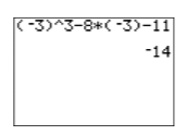
Given the polynomial function \(p(x)=x^{3}-8 x-11\), evaluate \(p(−3)\).

Solution

To evaluate \(p(−3)\), first restate the function definition, then replace each occurrence of the variable \(x\) with open parentheses.

\[\begin{aligned} p(x) &= x^{3}-8 x-11 \quad \color {Red} \text { Original function definition. } \\ p(\;\;) &= (\;\;)^{3}-8(\;\;)-11 \quad \color {Red} \text { Replace each occurrence of } x \text { with open parentheses. } \end{aligned} \nonumber \]

Next, substitute \(−3\) for \(x\) in the open parentheses prepared in the last step.

\[\begin{aligned} p(-3) &= (-3)^{3}-8(-3)-11 \quad \color {Red} \text { Substitute }-3 \text { for } x \text { in the open parentheses positions.} \\ p(-3) &= -27-8(-3)-11 \quad \color {Red} \text { Exponent first: }(-3)^{3}=-27 \\ p(-3) &= -27+24-11 \quad \color {Red} \text { Multiply: }-8(-3)=24 \\ p(-3) &= -14 \quad \color {Red} \text { Add. } \end{aligned} \nonumber \]

Hence, \(p(−3) = −14\). You can easily check this result on your calculator (see Figure \(\PageIndex{1}\)).

Figure \(\PageIndex{1}\): Calculator check.

Exercise \(\PageIndex{6}\)

Given the polynomial function \(p(x)=-3 x^{2}+7 x+4\), evaluate \(p(2)\).

Answer

\(6\)

The Graph of a Polynomial Function

One of the most important polynomial functions in all of mathematics and science is the polynomial having degree two.

Quadratic polynomial

The second degree polynomial having the form \[p(x)=a x^{2}+b x+c \nonumber \] is called a quadratic polynomial. The graph of this polynomial is called a parabola.

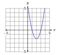
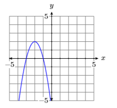
The parabola is approximately U-shaped. Some open upwards, some open downwards, depending on the sign of the leading term.

In Figure \(\PageIndex{2}\), the leading term of the parabola \(p(x)=2 x^{2}-8 x+6\) has positive two as its coefficient, so it opens upward.

Figure \(\PageIndex{2}\): The graph of \(p(x)=2 x^{2}-8 x+6\) opens up.

In Figure \(\PageIndex{3}\), the leading term of the parabola \(p(x)=-2 x^{2}-8 x-6\) has negative two as its coefficient, so it opens downward.

Figure \(\PageIndex{3}\): The graph of \(p(x)=-2 x^{2}-8 x-6\) opens down.

Note

The sign of the leading term of \(p(x)=ax^2 +bx+c\) determines whether the parabola opens up or down.

• If \(a>0\), the parabola opens upward.
• If \(a<0\), the parabola opens downward.

The turning point of a parabola has a special name.

The vertex of a parabola

The graph of the second degree polynomial \(p(x)=ax^2+bx+c\) has a single turning point, called the vertex of the parabola.

Example \(\PageIndex{7}\)

Use your graphing calculator to sketch the graph of the quadratic polynomial \(p(x)=−3x^2 + 12x + 25\).

Solution

The degree of the polynomial \(p(x)=−3x^2 + 12x + 25\) is two, so it is a quadratic polynomial and its graph is a parabola. Moreover, its leading term has negative three as its coefficient, so we know that the parabola opens downward. Enter \(y = −3x^2 + 12x + 25\) as \(Y 1=-3 * X \wedge 2+12 * X+25\) in the Y= menu (see the first image in Figure \(\PageIndex{4}\)), then select 6:ZStandard from the ZOOM menu to produce the third image in Figure \(\PageIndex{4}\).

Figure \(\PageIndex{4}\): Sketching the graph of \(p(x)=−3x^2 + 12x + 25\).

Note that the graph in Figure \(\PageIndex{4}\) appears to have the U-shape of a parabola that opens downwards. Its vertex (turning point) is not visible, but one would surmise that it lies off the top of the screen. We need to adjust the WINDOW parameters so that the vertex of the parabola is visible in the viewing screen. After some experimentation, we settle on the parameters shown in the first image in Figure \(\PageIndex{5}\), then push the GRAPH button to produce the second image in Figure \(\PageIndex{5}\).

Figure \(\PageIndex{5}\): Adjust the WINDOW parameters so that the vertex is visible in the viewing screen.

In reporting your result on your homework, follow the Calculator Submission Guidelines from Chapter 3, Section2.

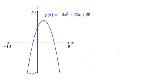
1. Draw axes with a ruler.
2. Label the horizontal axis \(x\) and the vertical axis \(y\).
3. Indicate the WINDOW parameters \(\mathrm{Xmin}, \mathrm{Xmax}, \mathrm{Ymin}\), and \(\mathrm{Ymax}\)\) at the end of each axis.
4. Freehand the curve and label it with its equation.

Exercise \(\PageIndex{7}\)

Use your graphing calculator to sketch the graph of the quadratic polynomial \(p(x)=2x^2 −5x−4\).

Answer

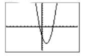
When the degree of the polynomial is larger than two, the number of turning points of the graph might increase. This makes for some very interesting curves. In more advanced courses, such as intermediate and college algebra, you will be introduced to a variety of techniques that will help you determine appropriate viewing windows for the graphs of these higher degree polynomials. However, in this introductory section, we will assist you by suggesting a good viewing window for each polynomial, one that will allow you to see all of the turning points of the graph of the polynomial.

Example \(\PageIndex{8}\)

Use your graphing calculator to sketch the graph of the polynomial function \(p(x)=x^{4}-37 x^{2}+24 x+180\). Set your window parameters as follows: \(\mathbf{X} \min =-10, \mathbf{X} \max =10, \mathbf{X} \operatorname{scl}=1, \mathbf{Y} \min =-1000, \mathbf{Y} \max = 1000,\) and \(\mathbf{Y} \operatorname{scl} =100\).

Solution

Enter the polynomial function in \(\mathbf{Y} \mathbf{1}\) of the Y= menu, then enter the suggested window parameters in the WINDOW menu (see Figure \(\PageIndex{6}\)).

Figure \(\PageIndex{6}\): Enter the polynomial and adjust the WINDOW parameters.

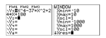
Push the GRAPH button on the top row of your calculator to produce the graph of the polynomial function shown in Figure \(\PageIndex{7}\).

Figure \(\PageIndex{7}\): The graph of \(p(x)=x^4 −37x^2 + 24x + 180\).

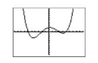
Sweet-looking curve!

Exercise \(\PageIndex{8}\)

Use your graphing calculator to sketch the graph of the quadratic polynomial p(x)=x3 −14x2 + 20x+ 60. Set your window parameters as follows: \(\mathbf{X} \min =-10, \mathbf{X} \max =20, \mathbf{X} \operatorname{scl}=1, \mathbf{Y} \min =-200, \mathbf{Y} \max = 200,\) and \(\mathbf{Y} \operatorname{scl} =20\).

Answer