6.2: Solving Nonlinear Equations

Last updated
Save as PDF

Page ID: 19885

$ \newcommand{\vecs}[1]{\overset { \scriptstyle \rightharpoonup} {\mathbf{#1}} } $

$ \newcommand{\vecd}[1]{\overset{-\!-\!\rightharpoonup}{\vphantom{a}\smash {#1}}} $

$ \newcommand{\id}{\mathrm{id}}$ $ \newcommand{\Span}{\mathrm{span}}$

( \newcommand{\kernel}{\mathrm{null}\,}\) $ \newcommand{\range}{\mathrm{range}\,}$

$ \newcommand{\RealPart}{\mathrm{Re}}$ $ \newcommand{\ImaginaryPart}{\mathrm{Im}}$

$ \newcommand{\Argument}{\mathrm{Arg}}$ $ \newcommand{\norm}[1]{\| #1 \|}$

$ \newcommand{\inner}[2]{\langle #1, #2 \rangle}$

$ \newcommand{\Span}{\mathrm{span}}$

$ \newcommand{\id}{\mathrm{id}}$

$ \newcommand{\Span}{\mathrm{span}}$

$ \newcommand{\kernel}{\mathrm{null}\,}$

$ \newcommand{\range}{\mathrm{range}\,}$

$ \newcommand{\RealPart}{\mathrm{Re}}$

$ \newcommand{\ImaginaryPart}{\mathrm{Im}}$

$ \newcommand{\Argument}{\mathrm{Arg}}$

$ \newcommand{\norm}[1]{\| #1 \|}$

$ \newcommand{\inner}[2]{\langle #1, #2 \rangle}$

$ \newcommand{\Span}{\mathrm{span}}$ $ \newcommand{\AA}{\unicode[.8,0]{x212B}}$

$ \newcommand{\vectorA}[1]{\vec{#1}} % arrow$

$ \newcommand{\vectorAt}[1]{\vec{\text{#1}}} % arrow$

$ \newcommand{\vectorB}[1]{\overset { \scriptstyle \rightharpoonup} {\mathbf{#1}} } $

$ \newcommand{\vectorC}[1]{\textbf{#1}} $

$ \newcommand{\vectorD}[1]{\overrightarrow{#1}} $

$ \newcommand{\vectorDt}[1]{\overrightarrow{\text{#1}}} $

$ \newcommand{\vectE}[1]{\overset{-\!-\!\rightharpoonup}{\vphantom{a}\smash{\mathbf {#1}}}} $

$ \newcommand{\vecs}[1]{\overset { \scriptstyle \rightharpoonup} {\mathbf{#1}} } $

$ \newcommand{\vecd}[1]{\overset{-\!-\!\rightharpoonup}{\vphantom{a}\smash {#1}}} $

$\newcommand{\avec}{\mathbf a}$ $\newcommand{\bvec}{\mathbf b}$ $\newcommand{\cvec}{\mathbf c}$ $\newcommand{\dvec}{\mathbf d}$ $\newcommand{\dtil}{\widetilde{\mathbf d}}$ $\newcommand{\evec}{\mathbf e}$ $\newcommand{\fvec}{\mathbf f}$ $\newcommand{\nvec}{\mathbf n}$ $\newcommand{\pvec}{\mathbf p}$ $\newcommand{\qvec}{\mathbf q}$ $\newcommand{\svec}{\mathbf s}$ $\newcommand{\tvec}{\mathbf t}$ $\newcommand{\uvec}{\mathbf u}$ $\newcommand{\vvec}{\mathbf v}$ $\newcommand{\wvec}{\mathbf w}$ $\newcommand{\xvec}{\mathbf x}$ $\newcommand{\yvec}{\mathbf y}$ $\newcommand{\zvec}{\mathbf z}$ $\newcommand{\rvec}{\mathbf r}$ $\newcommand{\mvec}{\mathbf m}$ $\newcommand{\zerovec}{\mathbf 0}$ $\newcommand{\onevec}{\mathbf 1}$ $\newcommand{\real}{\mathbb R}$ $\newcommand{\twovec}[2]{\left[\begin{array}{r}#1 \\ #2 \end{array}\right]}$ $\newcommand{\ctwovec}[2]{\left[\begin{array}{c}#1 \\ #2 \end{array}\right]}$ $\newcommand{\threevec}[3]{\left[\begin{array}{r}#1 \\ #2 \\ #3 \end{array}\right]}$ $\newcommand{\cthreevec}[3]{\left[\begin{array}{c}#1 \\ #2 \\ #3 \end{array}\right]}$ $\newcommand{\fourvec}[4]{\left[\begin{array}{r}#1 \\ #2 \\ #3 \\ #4 \end{array}\right]}$ $\newcommand{\cfourvec}[4]{\left[\begin{array}{c}#1 \\ #2 \\ #3 \\ #4 \end{array}\right]}$ $\newcommand{\fivevec}[5]{\left[\begin{array}{r}#1 \\ #2 \\ #3 \\ #4 \\ #5 \\ \end{array}\right]}$ $\newcommand{\cfivevec}[5]{\left[\begin{array}{c}#1 \\ #2 \\ #3 \\ #4 \\ #5 \\ \end{array}\right]}$ $\newcommand{\mattwo}[4]{\left[\begin{array}{rr}#1 \amp #2 \\ #3 \amp #4 \\ \end{array}\right]}$ $\newcommand{\laspan}[1]{\text{Span}\{#1\}}$ $\newcommand{\bcal}{\cal B}$ $\newcommand{\ccal}{\cal C}$ $\newcommand{\scal}{\cal S}$ $\newcommand{\wcal}{\cal W}$ $\newcommand{\ecal}{\cal E}$ $\newcommand{\coords}[2]{\left\{#1\right\}_{#2}}$ $\newcommand{\gray}[1]{\color{gray}{#1}}$ $\newcommand{\lgray}[1]{\color{lightgray}{#1}}$ $\newcommand{\rank}{\operatorname{rank}}$ $\newcommand{\row}{\text{Row}}$ $\newcommand{\col}{\text{Col}}$ $\renewcommand{\row}{\text{Row}}$ $\newcommand{\nul}{\text{Nul}}$ $\newcommand{\var}{\text{Var}}$ $\newcommand{\corr}{\text{corr}}$ $\newcommand{\len}[1]{\left|#1\right|}$ $\newcommand{\bbar}{\overline{\bvec}}$ $\newcommand{\bhat}{\widehat{\bvec}}$ $\newcommand{\bperp}{\bvec^\perp}$ $\newcommand{\xhat}{\widehat{\xvec}}$ $\newcommand{\vhat}{\widehat{\vvec}}$ $\newcommand{\uhat}{\widehat{\uvec}}$ $\newcommand{\what}{\widehat{\wvec}}$ $\newcommand{\Sighat}{\widehat{\Sigma}}$ $\newcommand{\lt}{<}$ $\newcommand{\gt}{>}$ $\newcommand{\amp}{&}$ $\definecolor{fillinmathshade}{gray}{0.9}$

We begin by introducing a property that will be used extensively in this and future sections.

The Zero Product Property

If the product of two or more numbers equals zero, then at least one of the numbers must equal zero. That is, if

$ab =0$

then

$a = 0$ or $b =0$

Let’s use the zero product property to solve a few equations.

Example $\PageIndex{1}$

Solve for $x$: $(x+3)(x-5)=0$

Solution

The product of two factors equals zero.

\[(x+3)(x-5)=0 \nonumber \]

Hence, at least one of the factors must equal zero. Using the zero product property, set each factor equal to zero, then solve the resulting equations for $x$.

\[\begin{aligned} x+3 &=0 \\ x &=-3 \end{aligned} \nonumber \]

\[\begin{aligned} x-5 &=0 \\ x &=5 \end{aligned} \nonumber \]

Hence, the solutions are $x = −3$ and $x =5$

Check:

Check that each solution satisﬁes the original equation.

Substitute $−3$ for $x$:

\[\begin{aligned}(x+3)(x-5) &=0 \\(-3+3)(-3-5) &=0 \\(0)(-8) &=0 \\ 0 &=0 \end{aligned} \nonumber \]

Substitute $5$ for $x$:

\[\begin{aligned}(x+3)(x-5) &=0 \\(5+3)(5-5) &=0 \\(8)(0) &=0 \\ 0 &=0 \end{aligned} \nonumber \]

Because each check produces a true statement, both $x = −3$ and $x = 5$ are solutions of $(x + 3)(x−5) = 0$.

Exercise $\PageIndex{1}$

Solve for x: $(x-7)(x-2)=0$

Answer: $7$, $2$

The zero product property also works equally well if more than two factors are present. For example, if $abc = 0$, then either $a = 0$ or $b = 0$ or $c = 0$. Let’s use this idea in the next example.

Example $\PageIndex{2}$

Solve for $x$: $x(2x + 9)(3x−5) = 0$

Solution

The product of three factors equals zero.

\[x(2x + 9)(3x−5) = 0 \nonumber \]

Using the zero product property, set each factor equal to zero, then solve the resulting equations for $x$.

\[x=0 \nonumber \]

\[\begin{align*} 2x + 9 &= 0\\ 2x &= -9\\ x &= -\dfrac{9}{2} \end{align*} \nonumber \]

\[\begin{align*} 3x - 5 &= 0\\ 3x &= 5\\ x &= \dfrac{5}{3} \end{align*} \nonumber \]

Hence, the solutions are $x = 0$, $x = −9/2$, and $x =5 /3$. We encourage the reader to check the solution.

Exercise $\PageIndex{2}$

Solve for $x$: $6x(x + 4)(5x + 1) = 0$

Answer: $0$, $−4$, $−1/5$

Linear versus Nonlinear

All of the equations solved in previous chapters were examples of what are called linear equations. If the highest power of the variable we are solving for is one, then the graphs involved are lines. Hence the term, linear equation. However, if the power on the variable we are solving for exceeds one, then the graphs involved are curves. Hence the term, nonlinear equation. In this chapter we will learn how to solve nonlinear equations involving polynomials. However, let’s ﬁrst make sure we can recognize the diﬀerence between a linear and a nonlinear equation.

Definition: Linear versus Nonlinear Equations

Use the following conditions to determine if an equation is linear or nonlinear.

If the highest power of the variable we are solving for is one, then the equation is linear.
If the highest power of the variable we are solving for is larger than one, then the equation is nonlinear.

Example $\PageIndex{3}$

If the instruction is “solve for $x$,” classify each of the following equations as linear or nonlinear.

$3x−5=4−7x$
$x^2 =8x$

Solution

Because the instruction is “solve for $x$,” to determine whether the equation is linear or nonlinear, we identify the largest power of $x$ present in the equation.

The highest power of $x$ present in the equation $3x− 5=4− 7x$ is one. Hence, this equation is linear.
The equation $x^2 =8 x$ contains a power of $x$ higher than one (it contains an $x^2$). Hence, this equation is nonlinear.

Exercise $\PageIndex{3}$

Classify the following equation as linear or nonlinear: $2x = x^3 −4$

Answer: nonlinear

Now that we can classify equations as either linear or nonlinear, let’s introduce strategies for solving each type, the ﬁrst of which should already be familiar.

Strategy for solving a linear equation

If an equation is linear, start the solution process by moving all terms containing the variable you are solving for to one side of the equation, then move all terms that do not contain the variable you are solving for to the other side of the equation.

Example $\PageIndex{4}$

Solve for $x$: $3 x−5=4−7x$

Solution

Because the instruction is “solve for $x$” and we note that the largest power of $x$ present is one, the equation $3x−5=4−7x$ is linear. Hence, the strategy is to move all terms containing $x$ to one side of the equation, then move all the remaining terms to the other side of the equation.

\[\begin{array}{rlrl}{3 x-5} & {=4-7 x} & {\color {Red} \text { Original equation. }} \\ {3 x-5+7 x} & {=4} & {\color {Red} \text { Add } 7 x \text { to both sides. }} \\ {3 x+7 x} & {=4+5} & {\color {Red} \text { Add } 5 \text { to both sides. }}\end{array} \nonumber \]

Note how we have succeeded in moving all terms containing $x$ to one side of the equation and all terms that do not contain $x$ to the other side of the equation.

\[\begin{array}{rlrl}{10 x} & {=9} & {} & {\color {Red} \text { Simplify both sides. }} \\ {x} & {=\dfrac{9}{10}} & {} & {\color {Red} \text { Divide both sides by } 10 .}\end{array} \nonumber \]

Hence, the solution of $3x−5=4−7x$ is $x =9 /10$. Readers are encouraged to check this solution.

Exercise $\PageIndex{4}$

Add exercises text here.

Answer: $1/4$

The situation is much diﬀerent when the equation is nonlinear.

Strategy for solving a nonlinear equation

If an equation is nonlinear, ﬁrst move everything to one side of the equation, making one side of the equation equal to zero. Continue the solution process by factoring and applying the zero product property.

Example $\PageIndex{5}$

Solve for $x$: $x^2 = 8x$

Solution

Because the instruction is “solve for $x$,” and the highest power of $x$ is larger than one, the equation $x^2 =8x$ is nonlinear. Hence, the strategy requires that we move all terms to one side of the equation, making one side zero.

\[\begin{array}{rlrl}{x^{2}} & {=8 x} \quad {\color {Red} \text { Original equation. }} \\ {x^{2}-8 x} & {=0} \quad {\color {Red} \text { Subtract } 8 x \text { from both sides. }}\end{array} \nonumber \]

Note how we have succeeded in moving all terms to one side of the equation, making one side equal to zero. To ﬁnish the solution, we factor out the $\mathrm{GCF}$ on the left-hand side.

\[x(x-8) = 0 \quad \color {Red} \text {Factor out the GCF.} \nonumber \]

Note that we now have a product of two factors that equals zero. By the zero product property, either the ﬁrst factor is zero or the second factor is zero.

\[\begin{array}{r}{x=0 \quad \text { or } \quad x-8=0} \\ {x=8}\end{array} \nonumber \]

Hence, the solutions are $x = 0$ and $x = 8$.

Check:

Check that each solution satisﬁes the original equation.

\[\begin{array}{l}{\text { Substitute } 0 \text { for } x :} \\ {\qquad \begin{aligned} x^{2} &=8 x \\(0)^{2} &=8(0) \\ 0 &=0 \end{aligned}}\end{array} \nonumber \]

\[\begin{array}{l}{\text { Subtitute } 8 \text { for } x :} \\ {\qquad \begin{aligned} x^{2} &=8 x \\(8)^{2} &=8(8) \\ 64 &=64 \end{aligned}}\end{array} \nonumber\]

Note that both results are true statements, guaranteeing that both $x = 0$ and $x = 8$ are solutions of $x^2 =8x$

Exercise $\PageIndex{5}$

Solve for $x$: $x^2 =−5x$

Answer: $0$, $-5$

Warning!

The following is incorrect!

Consider what would happen if we divided both sides of the equation $x^2 =8x$ in Example $\PageIndex{5}$ by $x$:

\[\begin{aligned} x^{2} &=8 x \\ \dfrac{x^{2}}{x} &=\dfrac{8 x}{x} \\ x &=8 \end{aligned} \nonumber \]

Note that we have lost the second answer found in Example $\PageIndex{5}$, $x = 0$. This example demonstrates that you should never divide by the variable you are solving for! If you do, and cancellation occurs, you will lose answers.

Let’s try solving a nonlinear equation that requires factoring by grouping.

Example $\PageIndex{6}$

Solve for $x$: $6x^2 +9x−8x−12 = 0$

Solution

Because we are solving for $x$ and there is a power of $x$ larger than one, this equation is nonlinear. Hence, the ﬁrst step is to move everything to one side of the equation, making one side equal to zero. Well that’s already done, so let’s factor the left-hand side by grouping. Note that we can factor $3x$ out of the ﬁrst two terms and $−4$ out of the second two terms.

$fig 6.2.a.png$

Factor out the common factor $2x + 3$.

\[(3x-4){\color {Red}(2x + 3)}=0 \nonumber \]

We now have a product of two factors that equals zero. Use the zero product property to write:

\[\begin{aligned} 3x-4 &=0 \\ 3x &= 4 \\ x &=\dfrac{4}{3} \end{aligned} \nonumber \]

\[\begin{aligned} 2x+3 &=0 \\ 2x &= -3 \\ x &= -\dfrac{3}{2} \end{aligned}\]

Hence, the solutions are $x =4 /3$ and $x =−3/2$.

Check:

Let’s use the graphing calculator to check the solution $x =4 /3$. First, store the solution $4/3$ in the variable $\mathbb{X}$ using the following keystrokes (see the ﬁrst image in Figure $\PageIndex{1}$.

fig 6.2.b.png — Figure $\PageIndex{1}$ indicates that the expression $6x^2 +9x−8x−12$ equals zero when $x =4 /3$.

fig 6.2.1.png — Figure $\PageIndex{1}$: Checking the solution $x =4 /3$.

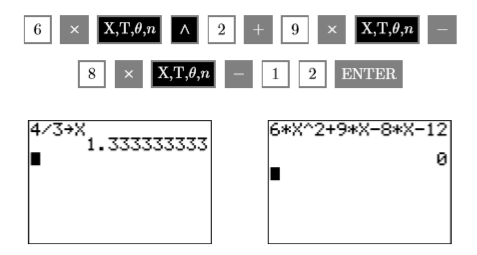
Therefore, the solution $x =4 /3$ checks. Readers are encouraged to use their graphing calculators to check the second solution, $x = −3/2$.

Exercise $\PageIndex{6}$

Solve for $x$: $5x^2 −20x−4x + 16 = 0$

Answer: $4/5$, $4$

Using the Graphing Calculator

In this section we will employ two diﬀerent calculator routines to ﬁnd the solution of a nonlinear equation. Before picking up the calculator, let’s ﬁrst use an algebraic method to solve the equation $x^2 = −5x$. The equation is nonlinear, so the ﬁrst step is to move everything to one side of the equation, making one side equal to zero.

\[\begin{aligned} x^{2} &= -5x \quad \color {Red} \text { Nonlinear. Make one side zero. } \\ x^{2}+5 x &= 0 \quad \color {Red} \text { Add } 5x \text { to both sides. } \\ x(x+5) &= 0 \quad \color {Red} \text { Factor out the GCF. } \end{aligned} \nonumber \]

Use the zero product property, setting each factor equal to zero, then solving the resulting equations for $x$.

\[x=0 \nonumber \]

\[\begin{aligned} x+5&=0 \\ x&=-5 \end{aligned} \nonumber \]

Hence, the solutions are $x = 0$ and $x = −5$.

We’ll now use the calculator to ﬁnd the solutions of $x^2 = −5x$. The ﬁrst technique employs the 5:intersect routine on the calculator’s CALC menu.

Example $\PageIndex{7}$

Use the 5:intersect utility on the graphing calculator to solve the equation $x^2 = −5x$ for $x$.

Solution

Load the left-hand side of $x^2 = −5x$ in $\mathbb{Y1}$ and the right-hand side in $\mathbb{Y2}$ (see Figure $\PageIndex{2}$). Selecting 6:ZStandard from the ZOOM menu produces the graphs shown in the image on the right in Figure $\PageIndex{2}$.

fig 6.2.2.png — Figure $\PageIndex{2}$: Sketch the graphs of each side of the equation $x^2 = −5x$.

Note that the graph of $y = x^2$ is a parabola that opens upward, with vertex (turning point) at the origin. This graph reveals why the equation $x^2 = −5x$ is called a nonlinear equation (not all the graphs involved are lines). Next, the graph of $y = −5x$ is a line with slope $−5$ and $y$-intercept at the origin.

The two graphs obviously intersect at the origin, but it also appears that there may be another point of intersection that is oﬀ the screen. Let’s increase $\mathbb{Ymax}$ in an attempt to reveal the second point of intersection. After some experimentation, the settings shown in the ﬁrst image in Figure $\PageIndex{3}$ reveal both points of intersection. Pushing the GRAPH button produces the image on the right in Figure $\PageIndex{3}$.

fig 6.2.3.png — Figure $\PageIndex{3}$: Adjust the **WINDOW** parameters to reveal both points of intersection.

To ﬁnd the solutions of the equation $x^2 =−5x$, we must ﬁnd the coordinates of the points where the graphs of $y = x^2$ and $y = −5x$ intersect. The $x$-coordinate of each point of intersection will be a solution of the equation $x^2 = −5x$.

Start by selecting 5:intersect from the CALC menu. When prompted for the “First curve?”, press ENTER. When prompted for the “Second curve?”, press ENTER. When prompted for a “Guess,” press ENTER. The result is the point $(0,0)$ shown in the image on the left in Figure $\PageIndex{4}$.
Repeat the process a second time. Select 5:intersect from the CALC menu. When prompted for the “First curve?”, press ENTER. When prompted for the “Second curve?”, press ENTER. When prompted for a “Guess,” use the left-arrow key to move the cursor closer to the leftmost point of intersection, then press ENTER. The result is the point $(−5,25)$ shown in the image on the right in Figure $\PageIndex{4}$.

fig 6.2.4.png — Figure $\PageIndex{4}$: Use the 5:intersect utility to ﬁnd the points of intersection.

Reporting the solution on your homework:

Duplicate the image in your calculator’s viewing window on your homework page. Use a ruler to draw all lines, but freehand any curves.

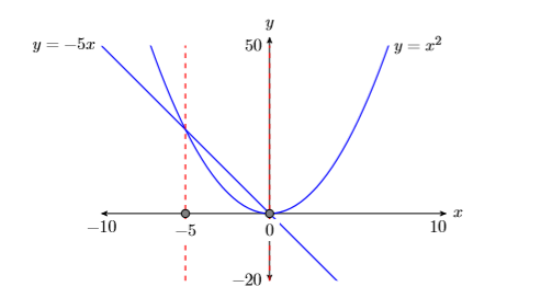
fig 6.2.5.png — Figure $\PageIndex{5}$: Reporting your graphical solution on your homework.

Label the horizontal and vertical axes with $x$ and $y$, respectively (see Figure $\PageIndex{5}$).
Place your WINDOW parameters at the end of each axis (see Figure $\PageIndex{5}$).
Label each graph with its equation (see Figure $\PageIndex{5}$).
Drop dashed vertical lines through each point of intersection. Shade and label the $x$-values of the points where the dashed vertical line crosses the $x$-axis. These are the solutions of the equation $x^2 =−5x$ (see Figure $\PageIndex{5}$).

Hence, the solutions of $x^2 = −5x$ are $x = −5$ and $x = 0$. Note now these match the solutions found using the algebraic technique.

Exercise $\PageIndex{7}$

Use the 5:intersect utility on the graphing calculator to solve the equation $x^2 =4x$ for $x$.

Answer: $Exercise 6.2.4.png$

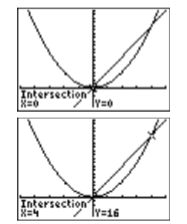
Before demonstrating a second graphing calculator technique for solving nonlinear equations, let’s take a moment to recall the deﬁnition of a zero of a function, which was ﬁrst presented in Chapter 5, Section 3.

Zeros and $x$-intercepts

The points where the graph of $f$ crosses the $x$-axis are called the $x$-intercepts of the graph of $f$. The $x$-value of each $x$-intercept is called a zero of the function $f$.

We’ll now employ the 2:zero utility from the CALC menu to ﬁnd the solutions of the equation $x^2 = −5x$.

Example $\PageIndex{8}$

Use the 2:zero utility on the graphing calculator to solve the equation $x^2 = −5x$ for $x$.

Solution

First, make one side of the equation equal to zero.

\[\begin{aligned}x^{2} &=-5 x \quad \color {Red} \text { Make one side zero. } \\ x^{2}+5 x &=0 \quad \color {Red} \text { Add } 5 x \text { to both sides. }\end{aligned} \nonumber \]

To determine the values of $x$ that make $x^2 +5x = 0$, we must locate the points where the graph of $f(x)=x^2 +5x$ crosses the $x$-axis. These points are the $x$-intercepts of the graph of $f$ and the $x$-values of these points are the zeros of the function $f$.

Load the function $f(x)=x^2 +5 x$ in $\mathbb{Y1}$, then select 6:ZStandard to produce the image in Figure $\PageIndex{6}$. Note that the graph of $f$ has two $x$-intercepts, and the $x$-values of each of these points are the zeros of the function $f$.

fig 6.2.6.png — Figure $\PageIndex{6}$: Sketch the graph of $p(x)=x^2 +5x$.

Note

It’s often easier to ﬁnd the solutions of a nonlinear equation by making one side zero and identifying where the graph of the resulting function crosses the $x$-axis.

Select 2:zero from the CALC menu (see Figure $\PageIndex{7}$).

fig 6.2.7.png — Figure $\PageIndex{7}$: Setting the left and right bounds when using the **2:zero** utility to ﬁnd the $x$-intercepts of the graph of $f(x)=x^2 +5x$.

The calculator responds by asking for a “Left Bound?” Use the left-arrow key to move the cursor so that it lies to the left of the $x$-intercept near $(−5,0)$ (see the second image in Figure $\PageIndex{7}$), then press the ENTER key.
The calculator responds by asking for a “Right Bound?” Move the cursor so that is slightly to the right of the x-intercept near $(−5,0)$ (see the third image Figure $\PageIndex{7}$), then press the ENTER key.
The calculator responds by asking for a “Guess?” Note the two triangular marks near the top of the viewing window in the ﬁrst image in Figure $\PageIndex{8}$ that mark the left- and right-bounds. As long as you place the cursor so that the x-value of the cursor location lies between these two marks, you’ve made a valid guess. Because the cursor already lies between these two marks, we usually leave it where it is and press the ENTER key.

fig 6.2.8.png — Figure $\PageIndex{8}$: *Setting the right bound and making a guess.*

After making your guess and pressing the ENTER key, the calculator proceeds to ﬁnd an approximation of the $x$-intercept that lies between the left- and right-bounds previously marked (see the second image in Figure $\PageIndex{8}$. Hence, this $x$-intercept is $(−5,0)$, making $−5$ a zero of $f(x)=x^2 +5x$ and a solution of the equation $x^2 +5x = 0$.

We’ll leave it to our readers to repeat the 2:zero process to ﬁnd the second zero at the origin.

Reporting the solution on your homework:

Duplicate the image in your calculator’s viewing window on your homework page. Use a ruler to draw all lines, but freehand any curves.

Label the horizontal and vertical axes with $x$ and $y$, respectively (see Figure $\PageIndex{9}$).
Place your WINDOW parameters at the end of each axis (see Figure $\PageIndex{9}$).
Label each graph with its equation (see Figure $\PageIndex{9}$).
Drop dashed vertical lines through each $x$-intercept. Shade and label the $x$-values of each $x$-intercept. These are the solutions of the equation $x^2 = −5x$ (see Figure $\PageIndex{9}$).

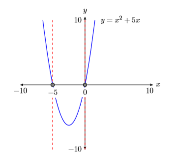
fig 6.2.9.png — Figure $\PageIndex{9}$: Reporting your graphical solution on your homework.

Hence, the solutions of $x^2 = −5x$ are $x = −5$ and $x = 0$. Note how nicely this agrees with the solutions found using the algebraic technique and the solutions found using the 5:intersect utility in Example $\PageIndex{7}$.

Exercise $\PageIndex{8}$

Use the 2:zero utility on the graphing calculator to solve the equation $x^2 =4x$ for $x$.

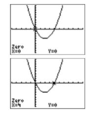
Answer: $Exercise 6.2.8.png$

Search

Text Color

Text Size

Margin Size

Font Type