5.2: Introduction to Polynomials

Last updated
Save as PDF

Page ID: 18355

Anonymous
LibreTexts

$ \newcommand{\vecs}[1]{\overset { \scriptstyle \rightharpoonup} {\mathbf{#1}} } $

$ \newcommand{\vecd}[1]{\overset{-\!-\!\rightharpoonup}{\vphantom{a}\smash {#1}}} $

$ \newcommand{\id}{\mathrm{id}}$ $ \newcommand{\Span}{\mathrm{span}}$

( \newcommand{\kernel}{\mathrm{null}\,}\) $ \newcommand{\range}{\mathrm{range}\,}$

$ \newcommand{\RealPart}{\mathrm{Re}}$ $ \newcommand{\ImaginaryPart}{\mathrm{Im}}$

$ \newcommand{\Argument}{\mathrm{Arg}}$ $ \newcommand{\norm}[1]{\| #1 \|}$

$ \newcommand{\inner}[2]{\langle #1, #2 \rangle}$

$ \newcommand{\Span}{\mathrm{span}}$

$ \newcommand{\id}{\mathrm{id}}$

$ \newcommand{\Span}{\mathrm{span}}$

$ \newcommand{\kernel}{\mathrm{null}\,}$

$ \newcommand{\range}{\mathrm{range}\,}$

$ \newcommand{\RealPart}{\mathrm{Re}}$

$ \newcommand{\ImaginaryPart}{\mathrm{Im}}$

$ \newcommand{\Argument}{\mathrm{Arg}}$

$ \newcommand{\norm}[1]{\| #1 \|}$

$ \newcommand{\inner}[2]{\langle #1, #2 \rangle}$

$ \newcommand{\Span}{\mathrm{span}}$ $ \newcommand{\AA}{\unicode[.8,0]{x212B}}$

$ \newcommand{\vectorA}[1]{\vec{#1}} % arrow$

$ \newcommand{\vectorAt}[1]{\vec{\text{#1}}} % arrow$

$ \newcommand{\vectorB}[1]{\overset { \scriptstyle \rightharpoonup} {\mathbf{#1}} } $

$ \newcommand{\vectorC}[1]{\textbf{#1}} $

$ \newcommand{\vectorD}[1]{\overrightarrow{#1}} $

$ \newcommand{\vectorDt}[1]{\overrightarrow{\text{#1}}} $

$ \newcommand{\vectE}[1]{\overset{-\!-\!\rightharpoonup}{\vphantom{a}\smash{\mathbf {#1}}}} $

$ \newcommand{\vecs}[1]{\overset { \scriptstyle \rightharpoonup} {\mathbf{#1}} } $

$ \newcommand{\vecd}[1]{\overset{-\!-\!\rightharpoonup}{\vphantom{a}\smash {#1}}} $

$\newcommand{\avec}{\mathbf a}$ $\newcommand{\bvec}{\mathbf b}$ $\newcommand{\cvec}{\mathbf c}$ $\newcommand{\dvec}{\mathbf d}$ $\newcommand{\dtil}{\widetilde{\mathbf d}}$ $\newcommand{\evec}{\mathbf e}$ $\newcommand{\fvec}{\mathbf f}$ $\newcommand{\nvec}{\mathbf n}$ $\newcommand{\pvec}{\mathbf p}$ $\newcommand{\qvec}{\mathbf q}$ $\newcommand{\svec}{\mathbf s}$ $\newcommand{\tvec}{\mathbf t}$ $\newcommand{\uvec}{\mathbf u}$ $\newcommand{\vvec}{\mathbf v}$ $\newcommand{\wvec}{\mathbf w}$ $\newcommand{\xvec}{\mathbf x}$ $\newcommand{\yvec}{\mathbf y}$ $\newcommand{\zvec}{\mathbf z}$ $\newcommand{\rvec}{\mathbf r}$ $\newcommand{\mvec}{\mathbf m}$ $\newcommand{\zerovec}{\mathbf 0}$ $\newcommand{\onevec}{\mathbf 1}$ $\newcommand{\real}{\mathbb R}$ $\newcommand{\twovec}[2]{\left[\begin{array}{r}#1 \\ #2 \end{array}\right]}$ $\newcommand{\ctwovec}[2]{\left[\begin{array}{c}#1 \\ #2 \end{array}\right]}$ $\newcommand{\threevec}[3]{\left[\begin{array}{r}#1 \\ #2 \\ #3 \end{array}\right]}$ $\newcommand{\cthreevec}[3]{\left[\begin{array}{c}#1 \\ #2 \\ #3 \end{array}\right]}$ $\newcommand{\fourvec}[4]{\left[\begin{array}{r}#1 \\ #2 \\ #3 \\ #4 \end{array}\right]}$ $\newcommand{\cfourvec}[4]{\left[\begin{array}{c}#1 \\ #2 \\ #3 \\ #4 \end{array}\right]}$ $\newcommand{\fivevec}[5]{\left[\begin{array}{r}#1 \\ #2 \\ #3 \\ #4 \\ #5 \\ \end{array}\right]}$ $\newcommand{\cfivevec}[5]{\left[\begin{array}{c}#1 \\ #2 \\ #3 \\ #4 \\ #5 \\ \end{array}\right]}$ $\newcommand{\mattwo}[4]{\left[\begin{array}{rr}#1 \amp #2 \\ #3 \amp #4 \\ \end{array}\right]}$ $\newcommand{\laspan}[1]{\text{Span}\{#1\}}$ $\newcommand{\bcal}{\cal B}$ $\newcommand{\ccal}{\cal C}$ $\newcommand{\scal}{\cal S}$ $\newcommand{\wcal}{\cal W}$ $\newcommand{\ecal}{\cal E}$ $\newcommand{\coords}[2]{\left\{#1\right\}_{#2}}$ $\newcommand{\gray}[1]{\color{gray}{#1}}$ $\newcommand{\lgray}[1]{\color{lightgray}{#1}}$ $\newcommand{\rank}{\operatorname{rank}}$ $\newcommand{\row}{\text{Row}}$ $\newcommand{\col}{\text{Col}}$ $\renewcommand{\row}{\text{Row}}$ $\newcommand{\nul}{\text{Nul}}$ $\newcommand{\var}{\text{Var}}$ $\newcommand{\corr}{\text{corr}}$ $\newcommand{\len}[1]{\left|#1\right|}$ $\newcommand{\bbar}{\overline{\bvec}}$ $\newcommand{\bhat}{\widehat{\bvec}}$ $\newcommand{\bperp}{\bvec^\perp}$ $\newcommand{\xhat}{\widehat{\xvec}}$ $\newcommand{\vhat}{\widehat{\vvec}}$ $\newcommand{\uhat}{\widehat{\uvec}}$ $\newcommand{\what}{\widehat{\wvec}}$ $\newcommand{\Sighat}{\widehat{\Sigma}}$ $\newcommand{\lt}{<}$ $\newcommand{\gt}{>}$ $\newcommand{\amp}{&}$ $\definecolor{fillinmathshade}{gray}{0.9}$

Learning Objectives

Identify a polynomial and determine its degree.
Evaluate a polynomial for given values of the variables.
Evaluate a polynomial using function notation.

Definitions

A polynomial is a special algebraic expression with terms that consist of real number coefficients and variable factors with whole number exponents.

$\color{Cerulean}{Examples\:of\:polynomials:}$

$3x^{2}\quad 7xy+5\quad \frac{3}{2}x^{3}+3x^{2}-\frac{1}{2}x+1\quad 6x^{2}y-4xy^{3}-4xy^{3}+7$

Polynomials do not have variables in the denominator of any term.

$\color{Cerulean}{Examples\:that\:are\:not\:polynomials:}$

$\frac{2x^{2}}{y} \quad 5\sqrt{x}+5\quad 5x^{2}+3x^{-2}+7\quad \frac{2}{x}-\frac{5}{y}=3$

The degree of a term in a polynomial is defined to be the exponent of the variable, or if there is more than one variable in the term, the degree is the sum of their exponents. Recall that $x^{0}=1$; any constant term can be written as a product of $x^{0}$ and itself. Hence the degree of a constant term is $0$.

Table $\PageIndex{1}$
Term	Degree
$3x^{2}$	$2$
$6x^{2}y$	$2+1=3$
$7a^{2}b^{3}$	$2+3=5$
$8$	$0$, since $8=8x^{0}$
$2x$	$1$, since $x=x^{1}$

The degree of a polynomial is the largest degree of all of its terms.

Table $\PageIndex{2}$
Polynomial	Degree
$4x^{5}-3x^{3}+2x-1$	$5$
$6x^{2}y-5xy^{3}+7$	$4$, because $5xy^{3}$ has degree $4$.
$12x+54$	$1$, because $x=x^{1}$

We classify polynomials by the number of terms and the degree as follows:

Table $\PageIndex{3}$
Expression	Classification	Degree
$5x^{7}$	Monomial (one term)	$7$
$8x^{6}-1$	Binomial (two terms)	$6$
$-3x^{2}+x-1$	Trinomial (three terms)	$2$
$5x^{3}-2x^{2}+3x-6$	Polynomial (many terms)	$3$

In this text, we will call polynomials with four or more terms simply polynomials.

Example $\PageIndex{1}$

Classify and state the degree:

$7x^{2}−4x^{5}−1$.

Solution:

Here there are three terms. The highest variable exponent is $5$. Therefore, this is a trinomial of degree $5$.

Answer:

Trinomial; degree $5$

Example $\PageIndex{2}$

Classify and state the degree:

$12a^{5}bc^{3}$.

Solution:

Since the expression consists of only multiplication, it is one term, a monomial. The variable part can be written as $a^{5}b^{1}c^{3}$; hence its degree is $5+1+3=9$.

Answer:

Monomial; degree $9$

Example $\PageIndex{3}$

Classify and state the degree:

$4x^{2}y−6xy^{4}+5x^{3}y^{3}+4$.

Solution:

The term $4x^{2}y$ has degree $3$; $−6xy^{4}$ has degree $5; 5x^{3}y^{3}$ has degree $6$; and the constant term $4$ has degree $0$. Therefore, the polynomial has $4$ terms with degree $6$.

Answer:

Polynomial; degree $6$

Of particular interest are polynomials with one variable, where each term is of the form $a_{n}x^{n}$. Here $a_{n}$ is any real number and $n$ is any whole number. Such polynomials have the standard form

\[a_{n}x^{n}+a_{n-1}x^{n-1}+...+a_{1}x+a_{0}\]

Typically, we arrange terms of polynomials in descending order based on the degree of each term. The leading coefficient is the coefficient of the variable with the highest power, in this case, $a_{n}$.

Example $\PageIndex{4}$

Write in standard form:

$3x−4x^{2}+5x^{3}+7−2x^{4}$.

Solution:

Since terms are separated by addition, write the following:

$\begin{aligned} & 3x-4x^{2}+5x^{3}+7-2x^{4} \\ &=3x+(-4x^{2})+5x^{3}+7+(-2x^{4}) \end{aligned}$

In this form, we can see that the subtraction in the original corresponds to negative coefficients. Because addition is commutative, we can write the terms in descending order based on the degree of each term as follows:

$\begin{aligned} &=(-2x^{4})+5x^{3}+(-4x^{2})+3x+7 \\ &=-2x^{4}+5x^{3}-4x^{2}+3x+7 \end{aligned}$

Answer:

$-2x^{4}+5x^{3}-4x^{2}+3x+7$

We can further classify polynomials with one variable by their degree as follows:

Table $\PageIndex{4}$
Polynomial	Name
$5$	Constant (degree $0$ )
$2x+1$	Linear (degree $1$ )
$3x^{2}+5x-3$	Quadratic (degree $2$ )
$x^{3}+x^{2}+x+1$	Cubic (degree $3$ )
$7x^{4}+3x^{3}-7x+8$	Fourth-degree polynomial

In this text, we call any polynomial of degree $n≥4$ an $n$th-degree polynomial. In other words, if the degree is $4$, we call the polynomial a fourth-degree polynomial. If the degree is $5$, we call it a fifth-degree polynomial, and so on.

Evaluating Polynomials

Given the values for the variables in a polynomial, we can substitute and simplify using the order of operations.

Example $\PageIndex{5}$

Evaluate:

$3x−1$, where $x=−\frac{3}{2}$.

Solution:

First, replace the variable with parentheses and then substitute the given value.

Answer:

$-\frac{11}{2}$

Example $\PageIndex{6}$

Evaluate:

$3x^{2}+2x−1$, where $x=−1$.

Solution:

Answer:

$0$

Example $\PageIndex{7}$

Evaluate:

$−2a^{2}b+ab^{2}−7$, where $a=3$ and $b=−2$.

Solution:

Answer:

$41$

Example $\PageIndex{8}$

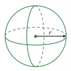
The volume of a sphere in cubic units is given by the formula $V=\frac{4}{3}πr^{3}$, where $r$ is the radius. Calculate the volume of a sphere with radius $r=\frac{3}{2}$ meters.

Screenshot (358).png — Figure $\PageIndex{1}$

Solution:

$\begin{aligned} V&=\frac{4}{3}\pi r^{3} \\ &=\frac{4}{3}\pi \left( \frac{3}{2} \right)^{3} \\ &=\frac{4}{3}\pi \frac{3^{3}}{2^{3}} \\ &=\frac{\color{Cerulean}{\stackrel{1}{\cancel{\color{black}{4}}}}}{\color{Cerulean}{\stackrel{\cancel{\color{black}{3}}}{1}}} \pi \frac{\color{Cerulean}{\stackrel{9}{\cancel{\color{black}{27}}}}}{\color{Cerulean}{\stackrel{\cancel{\color{black}{8}}}{2}}} \\ &=\frac{9}{2} \pi \end{aligned}$

Answer:

$\frac{9}{2}\pi$ cubic meters

Exercise $\PageIndex{1}$

Evaluate:

$x^{3}−x^{2}+4x−2$, where $x=−3$.

Answer: $-50$

Polynomial Functions

Polynomial functions with one variable are functions that can be written in the form

\[f(x) = a_{n}x^{n} + a_{n-1}x^{n-1} + ... + a_{0}\],

where $a_{n}$ is any real number and $n$ is any whole number. Some examples of the different classes of polynomial functions are listed below:

Table $\PageIndex{5}$
Polynomial function	Name
$f(x)=5$	Constant function (degree $0$ )
$f(x)=-2x+1$	Linear function (degree $1$ )
$f(x)=5x^{2}+4x-3$	Quadratic function (degree $2$ )
$f(x)=x^{3}-1$	Cubic function (degree $3$ )
$f(x)=4x^{5}+3x^{4}-7$	Polynomial function

Since there are no restrictions on the values for $x$, the domain of any polynomial function consists of all real numbers.

Example $\PageIndex{9}$

Calculate:

$f(5)$, given $f(x)=−2x^{2}+5x+10$.

Solution:

Recall that the function notation $f(5)$ indicates we should evaluate the function when $x=5$. Replace every instance of the variable $x$ with the value $5$.

Answer:

$f(5)=-15$

Example $\PageIndex{10}$

Calculate:

$f(−1)$, given $f(x)=−x^{3}+2x^{2}−4x+1$.

Solution:

Replace the variable $x$ with $−1$.

$\begin{aligned} f(\color{OliveGreen}{-1}\color{black}{)} &=-(\color{OliveGreen}{-1}\color{black}{)^{3}+2(}\color{OliveGreen}{-1}\color{black}{)^{2}-4(}\color{OliveGreen}{-1}\color{black}{)+1} \\ &=-(-1)+2\cdot 1 +4+1 \\ &=1+2+4+1 \\ &=8 \end{aligned}$

Answer:

$f(-1)=8$

Exercise $\PageIndex{2}$

Given $g(x)=x^{3}−2x^{2}−x−4$, calculate $g(−1)$.

Answer: $g(−1)=−6$

Key Takeaways

Polynomials are special algebraic expressions where the terms are the products of real numbers and variables with whole number exponents.
The degree of a polynomial with one variable is the largest exponent of the variable found in any term.
The terms of a polynomial are typically arranged in descending order based on the degree of each term.
When evaluating a polynomial, it is a good practice to replace all variables with parentheses and then substitute the appropriate values.
All polynomials are functions.

Exercise $\PageIndex{3}$ Definitions

Classify the given polynomial as linear, quadratic, or cubic.

$2x+1$
$x^{2}+7x+2$
$2−3x^{2}+x$
$4x$
$x^{2}−x^{3}+x+1$
$5−10x^{3}$

Answer

1. Linear

3. Quadratic

5. Cubic

Exercise $\PageIndex{4}$ Definitions

Classify the given polynomial as a monomial, binomial, or trinomial and state the degree.

$x^{3}−1$
$x^{2}y^{2}$
$x−x^{5}+1$
$x^{2}+3x−1$
$5ab^{4}$
$13x−12$
$−5x^{3}+2x+1$
$8x^{2}−9$
$4x^{5}−5x^{3}+6x$
$8x^{4}−x^{5}+2x−3$
$9x+7$
$x^{5}+x^{4}+x^{3}+x^{2}−x+1$
$6x−1+5x^{4}−8$
$4x−3x^{2}+3$
$7$
$x^{2}$
$4x^{2}y−3x^{3}y^{3}+xy^{3}$
$a^{3}b^{2}−6ab$
$a^{3}b^{3}$
$x^{2}y−y^{2}x$
$xy−3$
$a^{5}bc^{2}+3a^{9}−5a^{4}b^{3}c$
$−3x^{10}y^{2}z−xy^{12}z+9x^{13}+30$
$7x^{0}$

Answer

1. Binomial; degree $3$

3. Trinomial; degree $5$

5. Monomial; degree $5$

7. Trinomial; degree $3$

9. Trinomial; degree $5$

11. Binomial; degree $1$

13. Not a polynomial

15. Monomial; degree $0$

17. Trinomial; degree $6$

19. Monomial; degree $6$

21. Binomial; degree $2$

23. Polynomial; degree $14$

Exercise $\PageIndex{5}$ Definitions

Write the following polynomials in standard form.

$1−6x+7x^{2}$
$x−9x^{2}−8$
$7−x^{3}+x^{7}−x^{2}+x−5x^{5}$
$a^{3}−a^{9}+6a^{5}−a+3−a^{4}$

Answer

1. $7x^{2}−6x+1$

3. $x^{7}−5x^{5}−x^{3}−x^{2}+x+7$

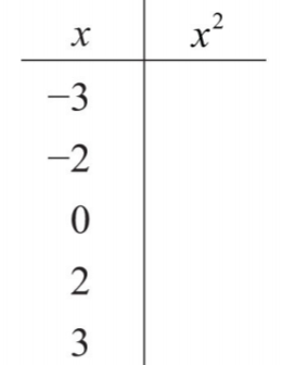
Exercise $\PageIndex{6}$ Evaluating Polynomials

Fill in the following chart:
$Screenshot (359).png$
Figure $\PageIndex{2}$
Fill in the following chart:
$Screenshot (360).png$
Figure $\PageIndex{3}$

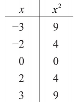
Answer: 1.

$Screenshot (361).png$
Figure $\PageIndex{4}$

Exercise $\PageIndex{7}$ Evaluating Polynomials

Evaluate.

$2x−3$, where $x=3$
$x^{2}−3x+5$, where $x=−2$
$−12x+13$, where $x=−13$
$−x^{2}+5x−1$, where $x=−12$
$−2x^{2}+3x−5$, where $x=0$
$8x^{5}−27x^{3}+81x−17$, where $x=0$
$y^{3}−2y+1$, where $y=−2$
$y^{4}+2y^{2}−32$, where $y=2$
$a^{3}+2a^{2}+a−3$, where $a=−3$
$x^{3}−x^{2}$, where $x=5$
$34x^{2}−12x+36$, where $x=−23$
$58x^{2}−14x+12$, where $x=4$
$x^{2}y+xy^{2}$, where $x=2$ and $y=−3$
$2a^{5}b−ab^{4}+a^{2}b^{2}$, where $a=−1$ and $b=−2$
$a^{2}−b^{2}$, where $a=5$ and $b=−6$
$a^{2}−b^{2}$, where $a=34$ and $b=−14$
$a^{3}−b^{3}$, where $a=−2$ and $b=3$
$a^{3}+b^{3}$, where $a=5$ and $b=−5$

Answer

1. $3$

3. $\frac{1}{2}$

5. $−5$

7. $−3$

9. $−15$

11. $\frac{7}{6}$

13. $6$

15. $−11$

17. $−35$

Exercise $\PageIndex{8}$ Evaluating Polynomials

For each problem, evaluate $b^{2}−4ac$, given the following values.

$a=−1, b=2$, and $c=−1$
$a=2, b=−2$, and $c=12$
$a=3, b=−5, c=0$
$a=1, b=0$, and $c=−4$
$a=14, b=−4$, and $c=2$
$a=1, b=5$, and $c=6$

Answer

1. $0$

3. $25$

5. $14$

Exercise $\PageIndex{9}$ Evaluating Polynomials

The volume of a sphere in cubic units is given by the formula $V=\frac{4}{3}πr^{3}$, where $r$ is the radius. For each problem, calculate the volume of a sphere given the following radii.

$r = 3$ centimeters
$r = 1$ centimeter
$r = \frac{1}{2}$ feet
$r = \frac{3}{2}$ feet
$r = 0.15$ in
$r = 1.3$ inches

Answer

1. $36π$ cubic centimeters

3. $\frac{π}{6}$ cubic feet

5. $0.014$ cubic inches

Exercise $\PageIndex{10}$ Evaluating Polynomials

The height in feet of a projectile launched vertically from the ground with an initial velocity $v_{0}$ in feet per second is given by the formula $h=−16t^{2}+v_{0}t$, where $t$ represents time in seconds. For each problem, calculate the height of the projectile given the following initial velocity and times.

$v_{0}=64$ feet/second, at times $t = 0, 1, 2, 3, 4$ seconds
$v_{0}=80$ feet/second, at times $t = 0, 1, 2, 2.5, 3, 4, 5$ seconds

Answer

Table $\PageIndex{6}$
Time	Height
$t=0$ seconds	$h=0$ feet
$t=1$ second	$h=48$ feet
$t=2$ seconds	$h=64$ feet
$t=3$ seconds	$h=48$ feet
$t=4$ seconds	$h=0$ feet

Exercise $\PageIndex{11}$ Evaluating Polynomials

The stopping distance of a car, taking into account an average reaction time, can be estimated with the formula $d=0.05v^{2}+1.5$, where $d$ is in feet and $v$ is the speed in miles per hour. For each problem, calculate the stopping distance of a car traveling at the given speeds.

$20$ miles per hour
$40$ miles per hour
$80$ miles per hour
$100$ miles per hour

Answer

1. $21.5$ feet

3. $321.5$ feet

Exercise $\PageIndex{12}$ Polynomial Functions

Given the linear function $f(x)=\frac{2}{3}x+6$, evaluate each of the following.

$f(−6)$
$f(−3)$
$f(0)$
$f(3)$
Find $x$ when $f(x)=10$.
Find $x$ when $f(x)=−4$.

Answer

1. $2$

3. $6$

5. $x=6$

Exercise $\PageIndex{13}$ Polynomial Functions

Given the quadratic function $f(x)=2x^{2}−3x+5$, evaluate each of the following.

$f(−2)$
$f(−1)$
$f(0)$
$f(2)$

Answer

1. $19$

3. $5$

Exercise $\PageIndex{14}$ Polynomial Functions

Given the cubic function $g(x)=x^{3}−x^{2}+x−1$, evaluate each of the following.

$g(−2)$
$g(−1)$
$g(0)$
$g(1)$

Answer

1. $-15$

3. $-1$

Exercise $\PageIndex{15}$ Polynomial Functions

The height in feet of a projectile launched vertically from the ground with an initial velocity of $128$ feet per second is given by the function $h(t)=−16t^{2}+128t$, where $t$ is in seconds. Calculate and interpret the following.

$h(0)$
$h(12) $
$h(1) $
$h(3) $
$h(4) $
$h(5) $
$h(7) $
$h(8)$

Answer

1. The projectile is launched from the ground.

3. The projectile is $112$ feet above the ground $1$ second after launch.

5. The projectile is $256$ feet above the ground $4$ seconds after launch.

7. The projectile is $112$ feet above the ground $7$ seconds after launch.

Exercise $\PageIndex{16}$ Discussion Board Topics

Find and share some graphs of polynomial functions.
Explain how to convert feet per second into miles per hour.
Find and share the names of fourth-degree, fifth-degree, and higher polynomials.

Answer

1. Answers may vary

3. Answers may vary

Term	Degree
\(3x^{2}\)	\(2\)
\(6x^{2}y\)	\(2+1=3\)
\(7a^{2}b^{3}\)	\(2+3=5\)
\(8\)	\(0\), since \(8=8x^{0}\)
\(2x\)	\(1\), since \(x=x^{1}\)

Polynomial	Degree
\(4x^{5}-3x^{3}+2x-1\)	\(5\)
\(6x^{2}y-5xy^{3}+7\)	\(4\), because \(5xy^{3}\) has degree \(4\).
\(12x+54\)	\(1\), because \(x=x^{1}\)

Expression	Classification	Degree
\(5x^{7}\)	Monomial (one term)	\(7\)
\(8x^{6}-1\)	Binomial (two terms)	\(6\)
\(-3x^{2}+x-1\)	Trinomial (three terms)	\(2\)
\(5x^{3}-2x^{2}+3x-6\)	Polynomial (many terms)	\(3\)

Polynomial	Name
\(5\)	Constant (degree \(0\) )
\(2x+1\)	Linear (degree \(1\) )
\(3x^{2}+5x-3\)	Quadratic (degree \(2\) )
\(x^{3}+x^{2}+x+1\)	Cubic (degree \(3\) )
\(7x^{4}+3x^{3}-7x+8\)	Fourth-degree polynomial

Polynomial function	Name
\(f(x)=5\)	Constant function (degree \(0\) )
\(f(x)=-2x+1\)	Linear function (degree \(1\) )
\(f(x)=5x^{2}+4x-3\)	Quadratic function (degree \(2\) )
\(f(x)=x^{3}-1\)	Cubic function (degree \(3\) )
\(f(x)=4x^{5}+3x^{4}-7\)	Polynomial function

Search

Text Color

Text Size

Margin Size

Font Type

Example \(\PageIndex{1}\)

Example \(\PageIndex{2}\)

Example \(\PageIndex{3}\)

Example \(\PageIndex{4}\)

Example \(\PageIndex{5}\)

Example \(\PageIndex{6}\)

Example \(\PageIndex{7}\)

Example \(\PageIndex{8}\)

Exercise \(\PageIndex{1}\)

Example \(\PageIndex{9}\)

Example \(\PageIndex{10}\)

Exercise \(\PageIndex{2}\)

Exercise \(\PageIndex{3}\) Definitions

Exercise \(\PageIndex{4}\) Definitions

Exercise \(\PageIndex{5}\) Definitions

Exercise \(\PageIndex{6}\) Evaluating Polynomials

Exercise \(\PageIndex{7}\) Evaluating Polynomials

Exercise \(\PageIndex{8}\) Evaluating Polynomials

Exercise \(\PageIndex{9}\) Evaluating Polynomials

Exercise \(\PageIndex{10}\) Evaluating Polynomials

Exercise \(\PageIndex{11}\) Evaluating Polynomials

Exercise \(\PageIndex{12}\) Polynomial Functions

Exercise \(\PageIndex{13}\) Polynomial Functions

Exercise \(\PageIndex{14}\) Polynomial Functions

Exercise \(\PageIndex{15}\) Polynomial Functions

Exercise \(\PageIndex{16}\) Discussion Board Topics

Time	Height
\(t=0\) seconds	\(h=0\) feet
\(t=1\) second	\(h=48\) feet
\(t=2\) seconds	\(h=64\) feet
\(t=3\) seconds	\(h=48\) feet
\(t=4\) seconds	\(h=0\) feet