
2.5: Solve Equations with Fractions or Decimals
- Page ID
- 15132

\( \newcommand{\vecs}[1]{\overset { \scriptstyle \rightharpoonup} {\mathbf{#1}} } \)
\( \newcommand{\vecd}[1]{\overset{-\!-\!\rightharpoonup}{\vphantom{a}\smash {#1}}} \)
\( \newcommand{\dsum}{\displaystyle\sum\limits} \)
\( \newcommand{\dint}{\displaystyle\int\limits} \)
\( \newcommand{\dlim}{\displaystyle\lim\limits} \)
\( \newcommand{\id}{\mathrm{id}}\) \( \newcommand{\Span}{\mathrm{span}}\)
( \newcommand{\kernel}{\mathrm{null}\,}\) \( \newcommand{\range}{\mathrm{range}\,}\)
\( \newcommand{\RealPart}{\mathrm{Re}}\) \( \newcommand{\ImaginaryPart}{\mathrm{Im}}\)
\( \newcommand{\Argument}{\mathrm{Arg}}\) \( \newcommand{\norm}[1]{\| #1 \|}\)
\( \newcommand{\inner}[2]{\langle #1, #2 \rangle}\)
\( \newcommand{\Span}{\mathrm{span}}\)
\( \newcommand{\id}{\mathrm{id}}\)
\( \newcommand{\Span}{\mathrm{span}}\)
\( \newcommand{\kernel}{\mathrm{null}\,}\)
\( \newcommand{\range}{\mathrm{range}\,}\)
\( \newcommand{\RealPart}{\mathrm{Re}}\)
\( \newcommand{\ImaginaryPart}{\mathrm{Im}}\)
\( \newcommand{\Argument}{\mathrm{Arg}}\)
\( \newcommand{\norm}[1]{\| #1 \|}\)
\( \newcommand{\inner}[2]{\langle #1, #2 \rangle}\)
\( \newcommand{\Span}{\mathrm{span}}\) \( \newcommand{\AA}{\unicode[.8,0]{x212B}}\)
\( \newcommand{\vectorA}[1]{\vec{#1}} % arrow\)
\( \newcommand{\vectorAt}[1]{\vec{\text{#1}}} % arrow\)
\( \newcommand{\vectorB}[1]{\overset { \scriptstyle \rightharpoonup} {\mathbf{#1}} } \)
\( \newcommand{\vectorC}[1]{\textbf{#1}} \)
\( \newcommand{\vectorD}[1]{\overrightarrow{#1}} \)
\( \newcommand{\vectorDt}[1]{\overrightarrow{\text{#1}}} \)
\( \newcommand{\vectE}[1]{\overset{-\!-\!\rightharpoonup}{\vphantom{a}\smash{\mathbf {#1}}}} \)
\( \newcommand{\vecs}[1]{\overset { \scriptstyle \rightharpoonup} {\mathbf{#1}} } \)
\(\newcommand{\longvect}{\overrightarrow}\)
\( \newcommand{\vecd}[1]{\overset{-\!-\!\rightharpoonup}{\vphantom{a}\smash {#1}}} \)
\(\newcommand{\avec}{\mathbf a}\) \(\newcommand{\bvec}{\mathbf b}\) \(\newcommand{\cvec}{\mathbf c}\) \(\newcommand{\dvec}{\mathbf d}\) \(\newcommand{\dtil}{\widetilde{\mathbf d}}\) \(\newcommand{\evec}{\mathbf e}\) \(\newcommand{\fvec}{\mathbf f}\) \(\newcommand{\nvec}{\mathbf n}\) \(\newcommand{\pvec}{\mathbf p}\) \(\newcommand{\qvec}{\mathbf q}\) \(\newcommand{\svec}{\mathbf s}\) \(\newcommand{\tvec}{\mathbf t}\) \(\newcommand{\uvec}{\mathbf u}\) \(\newcommand{\vvec}{\mathbf v}\) \(\newcommand{\wvec}{\mathbf w}\) \(\newcommand{\xvec}{\mathbf x}\) \(\newcommand{\yvec}{\mathbf y}\) \(\newcommand{\zvec}{\mathbf z}\) \(\newcommand{\rvec}{\mathbf r}\) \(\newcommand{\mvec}{\mathbf m}\) \(\newcommand{\zerovec}{\mathbf 0}\) \(\newcommand{\onevec}{\mathbf 1}\) \(\newcommand{\real}{\mathbb R}\) \(\newcommand{\twovec}[2]{\left[\begin{array}{r}#1 \\ #2 \end{array}\right]}\) \(\newcommand{\ctwovec}[2]{\left[\begin{array}{c}#1 \\ #2 \end{array}\right]}\) \(\newcommand{\threevec}[3]{\left[\begin{array}{r}#1 \\ #2 \\ #3 \end{array}\right]}\) \(\newcommand{\cthreevec}[3]{\left[\begin{array}{c}#1 \\ #2 \\ #3 \end{array}\right]}\) \(\newcommand{\fourvec}[4]{\left[\begin{array}{r}#1 \\ #2 \\ #3 \\ #4 \end{array}\right]}\) \(\newcommand{\cfourvec}[4]{\left[\begin{array}{c}#1 \\ #2 \\ #3 \\ #4 \end{array}\right]}\) \(\newcommand{\fivevec}[5]{\left[\begin{array}{r}#1 \\ #2 \\ #3 \\ #4 \\ #5 \\ \end{array}\right]}\) \(\newcommand{\cfivevec}[5]{\left[\begin{array}{c}#1 \\ #2 \\ #3 \\ #4 \\ #5 \\ \end{array}\right]}\) \(\newcommand{\mattwo}[4]{\left[\begin{array}{rr}#1 \amp #2 \\ #3 \amp #4 \\ \end{array}\right]}\) \(\newcommand{\laspan}[1]{\text{Span}\{#1\}}\) \(\newcommand{\bcal}{\cal B}\) \(\newcommand{\ccal}{\cal C}\) \(\newcommand{\scal}{\cal S}\) \(\newcommand{\wcal}{\cal W}\) \(\newcommand{\ecal}{\cal E}\) \(\newcommand{\coords}[2]{\left\{#1\right\}_{#2}}\) \(\newcommand{\gray}[1]{\color{gray}{#1}}\) \(\newcommand{\lgray}[1]{\color{lightgray}{#1}}\) \(\newcommand{\rank}{\operatorname{rank}}\) \(\newcommand{\row}{\text{Row}}\) \(\newcommand{\col}{\text{Col}}\) \(\renewcommand{\row}{\text{Row}}\) \(\newcommand{\nul}{\text{Nul}}\) \(\newcommand{\var}{\text{Var}}\) \(\newcommand{\corr}{\text{corr}}\) \(\newcommand{\len}[1]{\left|#1\right|}\) \(\newcommand{\bbar}{\overline{\bvec}}\) \(\newcommand{\bhat}{\widehat{\bvec}}\) \(\newcommand{\bperp}{\bvec^\perp}\) \(\newcommand{\xhat}{\widehat{\xvec}}\) \(\newcommand{\vhat}{\widehat{\vvec}}\) \(\newcommand{\uhat}{\widehat{\uvec}}\) \(\newcommand{\what}{\widehat{\wvec}}\) \(\newcommand{\Sighat}{\widehat{\Sigma}}\) \(\newcommand{\lt}{<}\) \(\newcommand{\gt}{>}\) \(\newcommand{\amp}{&}\) \(\definecolor{fillinmathshade}{gray}{0.9}\)By the end of this section, you will be able to:
- Solve equations with fraction coefficients
- Solve equations with decimal coefficients
Before you get started, take this readiness quiz.
- Multiply: \(8\cdot 38\).
If you missed this problem, review Exercise 1.6.16. - Find the LCD of \(\frac{5}{6}\) and \(\frac{1}{4}\).
If you missed this problem, review Exercise 1.7.16. - Multiply 4.78 by 100.
If you missed this problem, review Exercise 1.8.22.
Solve Equations with Fraction Coefficients
Let’s use the general strategy for solving linear equations introduced earlier to solve the equation, \(\frac{1}{8}x+\frac{1}{2}=\frac{1}{4}\).
 |
|
| To isolate the x term, subtract \(\frac{1}{2}\) from both sides. | 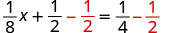 |
| Simplify the left side. | 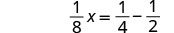 |
| Change the constants to equivalent fractions with the LCD. | 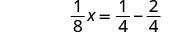 |
| Subtract. |  |
| Multiply both sides by the reciprocal of \(\frac{1}{8}\). |  |
| Simplify. |  |
This method worked fine, but many students do not feel very confident when they see all those fractions. So, we are going to show an alternate method to solve equations with fractions. This alternate method eliminates the fractions.
We will apply the Multiplication Property of Equality and multiply both sides of an equation by the least common denominator of all the fractions in the equation. The result of this operation will be a new equation, equivalent to the first, but without fractions. This process is called “clearing” the equation of fractions.
Let’s solve a similar equation, but this time use the method that eliminates the fractions.
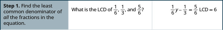
Solve: \(\frac{1}{6}y - \frac{1}{3} = \frac{5}{6}\)
Solution
Solve: \(\frac{1}{4}x + \frac{1}{2} = \frac{5}{8}\)
- Answer
-
\(x= \frac{1}{2}\)
Solve: \(\frac{1}{8}x + \frac{1}{2} = \frac{1}{4}\)
- Answer
-
\(x = -2\)
Notice in Exercise \(\PageIndex{1}\), once we cleared the equation of fractions, the equation was like those we solved earlier in this chapter. We changed the problem to one we already knew how to solve! We then used the General Strategy for Solving Linear Equations.
- Find the least common denominator of all the fractions in the equation.
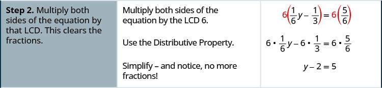
- Multiply both sides of the equation by that LCD. This clears the fractions.
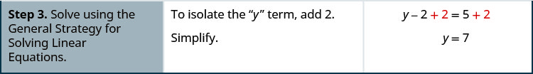
- Solve using the General Strategy for Solving Linear Equations.
Solve: \(6 = \frac{1}{2}v + \frac{2}{5}v - \frac{3}{4}v\)
Solution
We want to clear the fractions by multiplying both sides of the equation by the LCD of all the fractions in the equation.
| Find the LCD of all fractions in the equation. |  |
|
| The LCD is 20. | ||
| Multiply both sides of the equation by 20. |  |
|
| Distribute. | 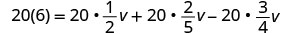 |
|
| Simplify—notice, no more fractions! |  |
|
| Combine like terms. |  |
|
| Divide by 3. | 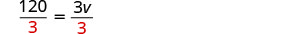 |
|
| Simplify. |  |
|
| Check: |  |
|
| Let v=40. |  |
|
 |
||
 |
||
Solve: \(7 = \frac{1}{2}x + \frac{3}{4}x - \frac{2}{3}x\)
- Answer
-
\(x = 12\)
Solve: \(-1 = \frac{1}{2}u + \frac{1}{4}u - \frac{2}{3}u\)
- Answer
-
\(u = -12\)
In the next example, we again have variables on both sides of the equation.
Solve: \(a + \frac{3}{4} = \frac{3}{8}a - \frac{1}{2}\)
Solution
 |
||
| Find the LCD of all fractions in the equation. The LCD is 8. |
||
| Multiply both sides by the LCD. |  |
|
| Distribute. | 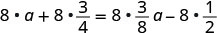 |
|
| Simplify—no more fractions. |  |
|
| Subtract 3a3a from both sides. |  |
|
| Simplify. |  |
|
| Subtract 6 from both sides. |  |
|
| Simplify. |  |
|
| Divide by 5. |  |
|
| Simplify. |  |
|
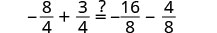
| Check: |  |
|
| Let a=−2. |  |
|
 |
||
 |
||
 |
||
Solve: \(x + \frac{1}{3} = \frac{1}{6}x - \frac{1}{2}\)
- Answer
-
\(x = -1\)
Solve: \(c + \frac{3}{4} = \frac{1}{2}c - \frac{1}{4}\)
- Answer
-
\(c = -2\)
In the next example, we start by using the Distributive Property. This step clears the fractions right away.
Solve: \(-5 = \frac{1}{4}(8x + 4)\)
Solution
 |
||
| Distribute. | 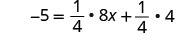 |
|
| Simplify. Now there are no fractions. |
 |
|
| Subtract 1 from both sides. |  |
|
| Simplify. |  |
|
| Divide by 2. | 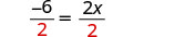 |
|
| Simplify. |  |
|
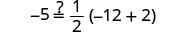
| Check: |  |
|
| Let x=−3. | 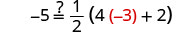 |
|
 |
||
 |
||
 |
||
Solve: \(-11 = \frac{1}{2}(6p + 2)\)
- Answer
-
\(p = -4\)
Solve: \(8 = \frac{1}{3}(9q + 6)\)
- Answer
-
\(q = 2\)
In the next example, even after distributing, we still have fractions to clear.
Solve: \(\frac{1}{2}(y - 5) = \frac{1}{4}(y - 1)\)
Solution
 |
||
| Distribute. | 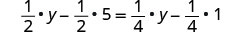 |
|
| Simplify. |  |
|
| Multiply by the LCD, 4. |  |
|
| Distribute. | 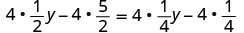 |
|
| Simplify. |  |
|
| Collect the variables to the left. |  |
|
| Simplify. |  |
|
| Collect the constants to the right. |  |
|
| Simplify. |  |
|
| Check: |  |
|
| Let y=9. |  |
|
| Finish the check on your own. | ||
Solve: \(\frac{1}{5}(n + 3) = \frac{1}{4}(n + 2)\)
- Answer
-
\(n = 2\)
Solve: \(\frac{1}{2}(m - 3) = \frac{1}{4}(m - 7)\)
- Answer
-
\(m = -1\)
Solve: \(\frac{5x - 3}{4} = \frac{x}{2}\)
Solution
 |
||
| Multiply by the LCD, 4. | 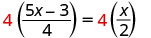 |
|
| Simplify. |  |
|
| Collect the variables to the right. |  |
|
| Simplify. |  |
|
| Divide. | 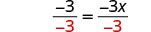 |
|
| Simplify. |  |
|
| Check: |  |
|
| Let x=1. | 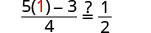 |
|
 |
||
 |
||
Solve: \(\frac{4y - 7}{3} = \frac{y}{6}\)
- Answer
-
\(y = 2\)
Solve: \(\frac{-2z - 5}{4} = \frac{z}{8}\)
- Answer
-
\(z = -2\)
Solve: \(\frac{a}{6} + 2 = \frac{a}{4} + 3\)
Solution
 |
||
| Multiply by the LCD, 12. | 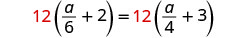 |
|
| Distribute. | 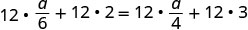 |
|
| Simplify. |  |
|
| Collect the variables to the right. |  |
|
| Simplify. |  |
|
| Collect the constants to the left. |  |
|
| Simplify. |  |
|
| Check: |  |
|
| Let a=−12. |  |
|
 |
||
 |
||
Solve: \(\frac{b}{10} + 2 = \frac{b}{4} + 5\)
- Answer
-
\(b = -20\)
Solve: \(\frac{c}{6} + 3 = \frac{c}{3} + 4\)
- Answer
-
\(c= -6\)
Solve: \(\frac{4q + 3}{2}+ 6 = \frac{3q + 5}{4}\)
Solution
 |
||
| Multiply by the LCD, 4. | 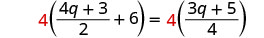 |
|
| Distribute. | 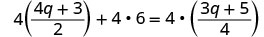 |
|
| Simplify. |    |
|
| Collect the variables to the left. |  |
|
| Simplify. |  |
|
| Collect the constants to the right. |  |
|
| Simplify. |  |
|
| Divide by 5. |  |
|
| Simplify. |  |
|
| Check: |  |
|
| Let q=−5. | 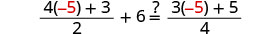 |
|
| Finish the check on your own. | ||
Solve: \(\frac{3r + 5}{6}+ 1 = \frac{4r + 3}{3}\)
- Answer
-
\(r = 1\)
Solve: \(\frac{2s + 3}{2}+ 1 = \frac{3s + 2}{4}\)
- Answer
-
\(s = -8\)
Solve Equations with Decimal Coefficients
Some equations have decimals in them. This kind of equation will occur when we solve problems dealing with money or percentages. But decimals can also be expressed as fractions. For example, \(0.3 = \frac{3}{10}\) and \(0.17 = \frac{17}{100}\). So, with an equation with decimals, we can use the same method we used to clear fractions—multiply both sides of the equation by the least common denominator.
Solve: \(0.06x + 0.02 = 0.25x - 1.5\)
Solution
Look at the decimals and think of the equivalent fractions.
\(0.06 = \frac { 6 } { 100 } \quad 0.02 = \frac { 2 } { 100 } \quad 0.25 = \frac { 25 } { 100 } \quad 1.5 = 1 \frac { 5 } { 10 }\)
Notice, the LCD is 100.
By multiplying by the LCD, we will clear the decimals from the equation.
 |
|
| Multiply both side by 100. |  |
| Distribute. |  |
| Multiply, and now we have no more decimals. |  |
| Collect the variables to the right. |  |
| Simplify. |  |
| Collect the variables to the right. |  |
| Simplify. |  |
| Divide by 19. |  |
| Simplify. |  |
Check: Let x=8 |
Solve: \(0.14h + 0.12 = 0.35h - 2.4\)
- Answer
-
\(h = 12\)
Solve: \(0.65k - 0.1 = 0.4k - 0.35\)
- Answer
-
\(k = -1\)
The next example uses an equation that is typical of the money applications in the next chapter. Notice that we distribute the decimal before we clear all the decimals.
Solve: \(0.25x + 0.05(x + 3) = 2.85\)
Solution
 |
|
| Distribute first. |  |
| Combine like terms. |  |
| To clear decimals, multiply by 100. |  |
| Distribute. |  |
| Subtract 15 from both sides. |  |
| Simplify. |  |
| Divide by 30. |  |
| Simplify. |  |
| Check it yourself by substituting x=9 into the original equation. |
Solve: \(0.25n + 0.05(n + 5) = 2.95\)
- Answer
-
\(n = 9\)
Solve: \(0.10d + 0.05(d -5) = 2.15\)
- Answer
-
\(d = 16\)
Key Concepts
- Strategy to Solve an Equation with Fraction Coefficients
- Find the least common denominator of all the fractions in the equation.
- Multiply both sides of the equation by that LCD. This clears the fractions.
- Solve using the General Strategy for Solving Linear Equations.