5.1: The Parabola
- Page ID
- 19706
\( \newcommand{\vecs}[1]{\overset { \scriptstyle \rightharpoonup} {\mathbf{#1}} } \)
\( \newcommand{\vecd}[1]{\overset{-\!-\!\rightharpoonup}{\vphantom{a}\smash {#1}}} \)
\( \newcommand{\dsum}{\displaystyle\sum\limits} \)
\( \newcommand{\dint}{\displaystyle\int\limits} \)
\( \newcommand{\dlim}{\displaystyle\lim\limits} \)
\( \newcommand{\id}{\mathrm{id}}\) \( \newcommand{\Span}{\mathrm{span}}\)
( \newcommand{\kernel}{\mathrm{null}\,}\) \( \newcommand{\range}{\mathrm{range}\,}\)
\( \newcommand{\RealPart}{\mathrm{Re}}\) \( \newcommand{\ImaginaryPart}{\mathrm{Im}}\)
\( \newcommand{\Argument}{\mathrm{Arg}}\) \( \newcommand{\norm}[1]{\| #1 \|}\)
\( \newcommand{\inner}[2]{\langle #1, #2 \rangle}\)
\( \newcommand{\Span}{\mathrm{span}}\)
\( \newcommand{\id}{\mathrm{id}}\)
\( \newcommand{\Span}{\mathrm{span}}\)
\( \newcommand{\kernel}{\mathrm{null}\,}\)
\( \newcommand{\range}{\mathrm{range}\,}\)
\( \newcommand{\RealPart}{\mathrm{Re}}\)
\( \newcommand{\ImaginaryPart}{\mathrm{Im}}\)
\( \newcommand{\Argument}{\mathrm{Arg}}\)
\( \newcommand{\norm}[1]{\| #1 \|}\)
\( \newcommand{\inner}[2]{\langle #1, #2 \rangle}\)
\( \newcommand{\Span}{\mathrm{span}}\) \( \newcommand{\AA}{\unicode[.8,0]{x212B}}\)
\( \newcommand{\vectorA}[1]{\vec{#1}} % arrow\)
\( \newcommand{\vectorAt}[1]{\vec{\text{#1}}} % arrow\)
\( \newcommand{\vectorB}[1]{\overset { \scriptstyle \rightharpoonup} {\mathbf{#1}} } \)
\( \newcommand{\vectorC}[1]{\textbf{#1}} \)
\( \newcommand{\vectorD}[1]{\overrightarrow{#1}} \)
\( \newcommand{\vectorDt}[1]{\overrightarrow{\text{#1}}} \)
\( \newcommand{\vectE}[1]{\overset{-\!-\!\rightharpoonup}{\vphantom{a}\smash{\mathbf {#1}}}} \)
\( \newcommand{\vecs}[1]{\overset { \scriptstyle \rightharpoonup} {\mathbf{#1}} } \)
\(\newcommand{\longvect}{\overrightarrow}\)
\( \newcommand{\vecd}[1]{\overset{-\!-\!\rightharpoonup}{\vphantom{a}\smash {#1}}} \)
\(\newcommand{\avec}{\mathbf a}\) \(\newcommand{\bvec}{\mathbf b}\) \(\newcommand{\cvec}{\mathbf c}\) \(\newcommand{\dvec}{\mathbf d}\) \(\newcommand{\dtil}{\widetilde{\mathbf d}}\) \(\newcommand{\evec}{\mathbf e}\) \(\newcommand{\fvec}{\mathbf f}\) \(\newcommand{\nvec}{\mathbf n}\) \(\newcommand{\pvec}{\mathbf p}\) \(\newcommand{\qvec}{\mathbf q}\) \(\newcommand{\svec}{\mathbf s}\) \(\newcommand{\tvec}{\mathbf t}\) \(\newcommand{\uvec}{\mathbf u}\) \(\newcommand{\vvec}{\mathbf v}\) \(\newcommand{\wvec}{\mathbf w}\) \(\newcommand{\xvec}{\mathbf x}\) \(\newcommand{\yvec}{\mathbf y}\) \(\newcommand{\zvec}{\mathbf z}\) \(\newcommand{\rvec}{\mathbf r}\) \(\newcommand{\mvec}{\mathbf m}\) \(\newcommand{\zerovec}{\mathbf 0}\) \(\newcommand{\onevec}{\mathbf 1}\) \(\newcommand{\real}{\mathbb R}\) \(\newcommand{\twovec}[2]{\left[\begin{array}{r}#1 \\ #2 \end{array}\right]}\) \(\newcommand{\ctwovec}[2]{\left[\begin{array}{c}#1 \\ #2 \end{array}\right]}\) \(\newcommand{\threevec}[3]{\left[\begin{array}{r}#1 \\ #2 \\ #3 \end{array}\right]}\) \(\newcommand{\cthreevec}[3]{\left[\begin{array}{c}#1 \\ #2 \\ #3 \end{array}\right]}\) \(\newcommand{\fourvec}[4]{\left[\begin{array}{r}#1 \\ #2 \\ #3 \\ #4 \end{array}\right]}\) \(\newcommand{\cfourvec}[4]{\left[\begin{array}{c}#1 \\ #2 \\ #3 \\ #4 \end{array}\right]}\) \(\newcommand{\fivevec}[5]{\left[\begin{array}{r}#1 \\ #2 \\ #3 \\ #4 \\ #5 \\ \end{array}\right]}\) \(\newcommand{\cfivevec}[5]{\left[\begin{array}{c}#1 \\ #2 \\ #3 \\ #4 \\ #5 \\ \end{array}\right]}\) \(\newcommand{\mattwo}[4]{\left[\begin{array}{rr}#1 \amp #2 \\ #3 \amp #4 \\ \end{array}\right]}\) \(\newcommand{\laspan}[1]{\text{Span}\{#1\}}\) \(\newcommand{\bcal}{\cal B}\) \(\newcommand{\ccal}{\cal C}\) \(\newcommand{\scal}{\cal S}\) \(\newcommand{\wcal}{\cal W}\) \(\newcommand{\ecal}{\cal E}\) \(\newcommand{\coords}[2]{\left\{#1\right\}_{#2}}\) \(\newcommand{\gray}[1]{\color{gray}{#1}}\) \(\newcommand{\lgray}[1]{\color{lightgray}{#1}}\) \(\newcommand{\rank}{\operatorname{rank}}\) \(\newcommand{\row}{\text{Row}}\) \(\newcommand{\col}{\text{Col}}\) \(\renewcommand{\row}{\text{Row}}\) \(\newcommand{\nul}{\text{Nul}}\) \(\newcommand{\var}{\text{Var}}\) \(\newcommand{\corr}{\text{corr}}\) \(\newcommand{\len}[1]{\left|#1\right|}\) \(\newcommand{\bbar}{\overline{\bvec}}\) \(\newcommand{\bhat}{\widehat{\bvec}}\) \(\newcommand{\bperp}{\bvec^\perp}\) \(\newcommand{\xhat}{\widehat{\xvec}}\) \(\newcommand{\vhat}{\widehat{\vvec}}\) \(\newcommand{\uhat}{\widehat{\uvec}}\) \(\newcommand{\what}{\widehat{\wvec}}\) \(\newcommand{\Sighat}{\widehat{\Sigma}}\) \(\newcommand{\lt}{<}\) \(\newcommand{\gt}{>}\) \(\newcommand{\amp}{&}\) \(\definecolor{fillinmathshade}{gray}{0.9}\)In this section you will learn how to draw the graph of the quadratic function defined by the equation
\[f(x)=a(x-h)^{2}+k \label{eq1} \]
You will quickly learn that the graph of the quadratic function is shaped like a "U" and is called a parabola. The form of the quadratic function in Equation \ref{eq1} is called vertex form, so named because the form easily reveals the vertex or “turning point” of the parabola. Each of the constants in the vertex form of the quadratic function plays a role. As you will soon see, the constant a controls the scaling (stretching or compressing of the parabola), the constant h controls a horizontal shift and placement of the axis of symmetry, and the constant \(k\) controls the vertical shift. Let’s begin by looking at the scaling of the quadratic.
Scaling the Quadratic
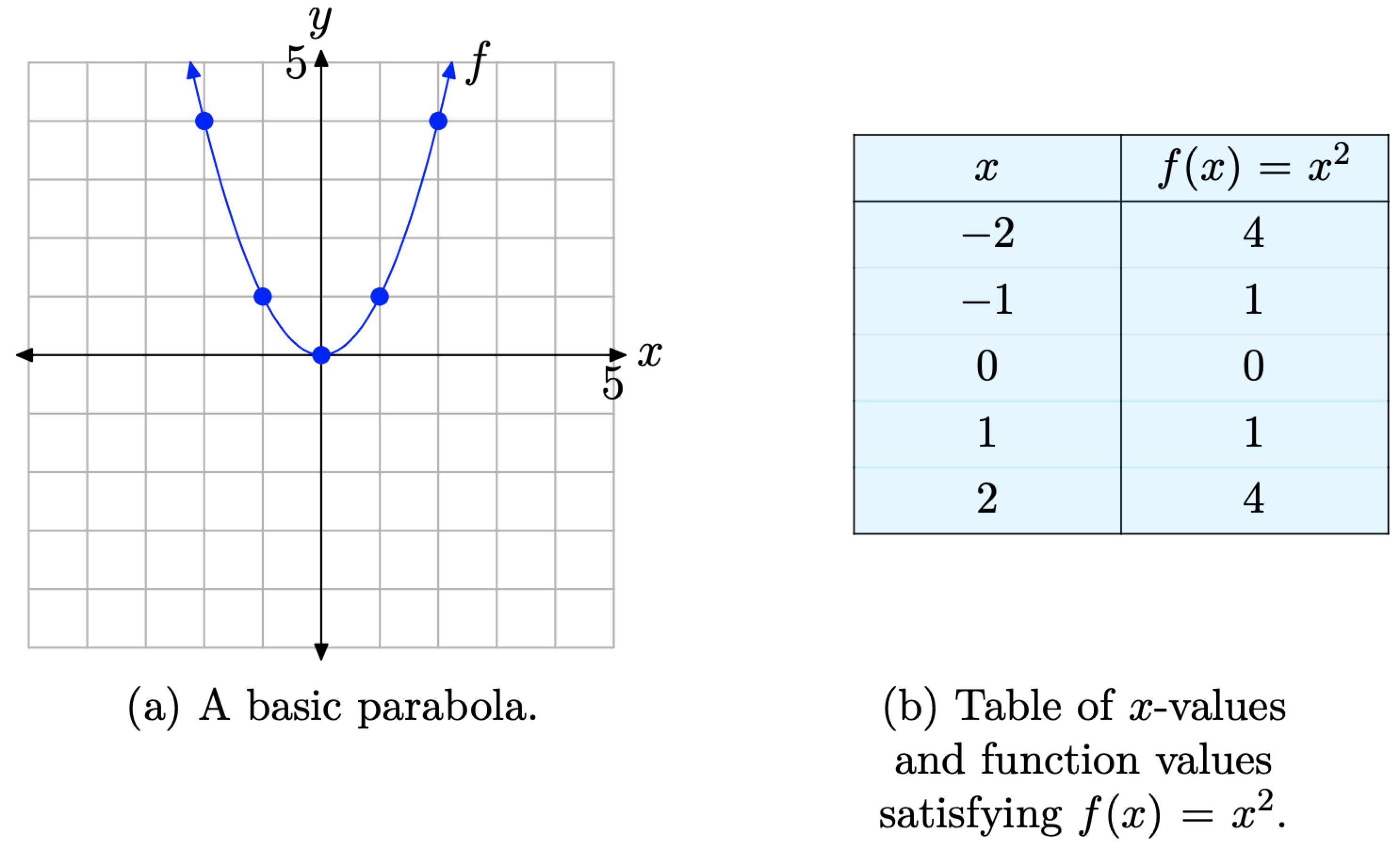
The graph of the basic quadratic function \(f(x)=x^{2}\) shown in Figure \(\PageIndex{1}\)(a) is a parabola. We say that the parabola in Figure \(\PageIndex{1}\)(a) “opens upward.” The point at (0, 0), the “turning point” of the parabola, is called the vertex of the parabola. We’ve tabulated a few points for reference in the table in Figure \(\PageIndex{1}\)(b) and then superimposed these points on the graph of \(f(x)=x^{2}\) in Figure \(\PageIndex{1}\)(a).
Now that we know the basic shape of the parabola determined by \(f(x) = x^{2}\), let’s see what happens when we scale the graph of \(f(x) = x^{2}\) in the vertical direction. For example, let’s investigate the graph of \(g(x) = 2x^{2}\). The factor of 2 has a doubling effect. Note that each of the function values of g is twice the corresponding function value of f in the table in Figure \(\PageIndex{2}\)(b).
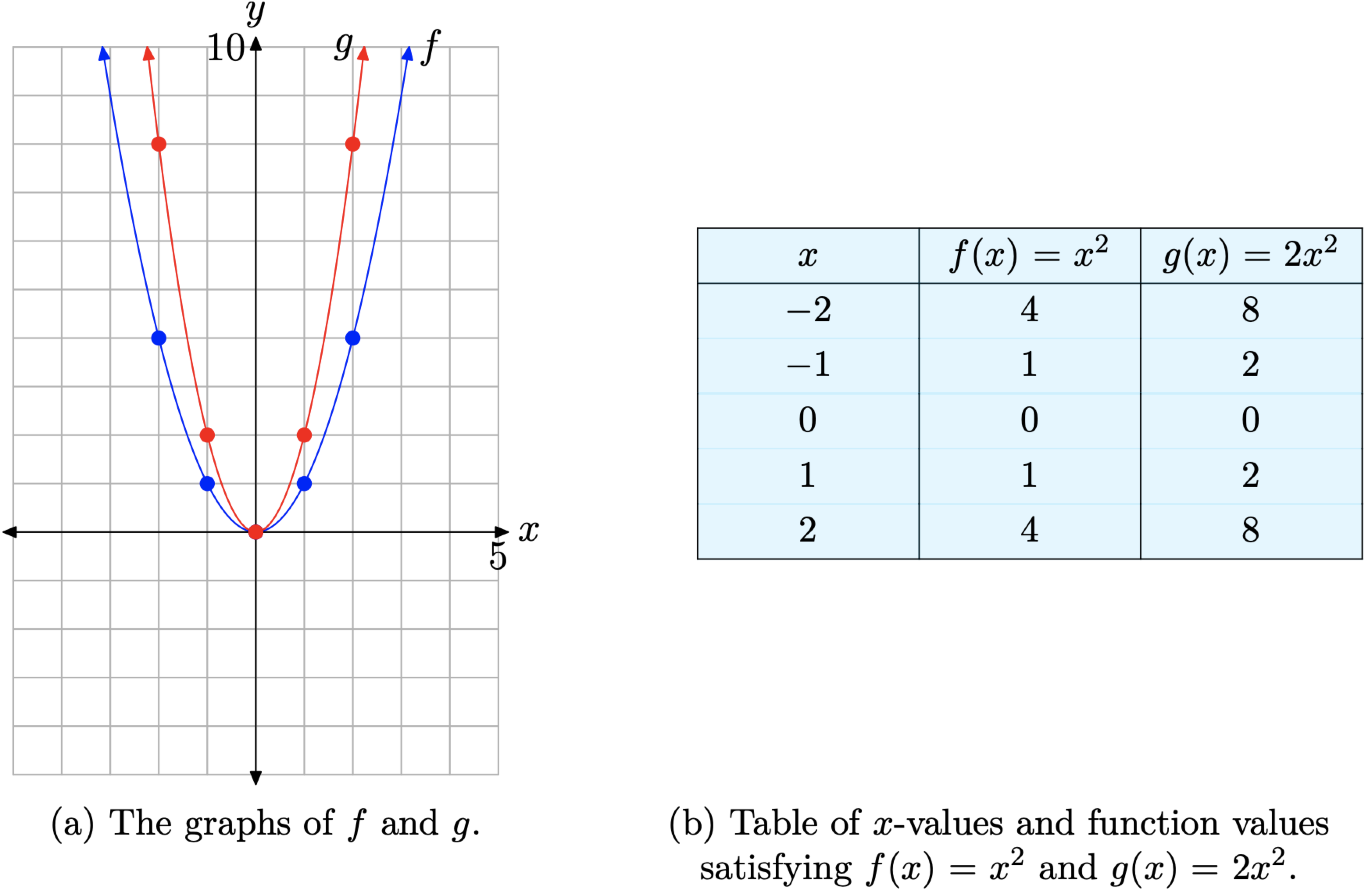
When the points in the table in Figure \(\PageIndex{2}\)(b) are added to the coordinate system in Figure \(\PageIndex{2}\)(a), the resulting graph of g is stretched by a factor of two in the vertical direction. It’s as if we had put the original graph of f on a sheet of rubber graph paper, grabbed the top and bottom edges of the sheet, and then pulled each edge in the vertical direction to stretch the graph of f by a factor of two. Consequently, the graph of \(g(x) = 2x^{2}\) appears somewhat narrower in appearance, as seen in comparison to the graph of \(f(x) = x^{2}\) in Figure \(\PageIndex{2}\)(a). Note, however, that the vertex at the origin is unaffected by this scaling.
In like manner, to draw the graph of \(h(x) = 3x^{2}\), take the graph of \(f(x) = x^{2}\) and stretch the graph by a factor of three, tripling the y-value of each point on the original graph of f. This idea leads to the following result.
If a is a constant larger than 1, that is, if \(a > 1\), then the graph of \(g(x) = ax^{2}\), when compared with the graph of \(f(x) = x^{2}\), is stretched by a factor of a.
Compare the graphs of \(y = x^{2}\), \(y = 2x ^{2}\), and \(y = 3x^{2}\) on your graphing calculator.
Solution
Load the functions \(y = x^{2}\), \(y = 2x ^{2}\), and \(y = 3x^{2}\) into the Y= menu, as shown in Figure \(\PageIndex{3}\)(a). Push the ZOOM button and select 6:ZStandard to produce the image shown in Figure \(\PageIndex{3}\)(b).
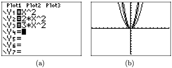
Note that as the “a” in \(y = ax^{2}\) increases from 1 to 2 to 3, the graph of \(y = ax^{2}\) stretches further and becomes, in a sense, narrower in appearance.
Next, let’s consider what happens when we scale by a number that is smaller than 1 (but greater than zero — we’ll deal with the negative in a moment). For example, let’s investigate the graph of \(g(x) = (1/2)x^{2}\). The factor 1/2 has a halving effect. Note that each of the function values of g is half the corresponding function value of f in the table in Figure \(\PageIndex{4}\)(b).
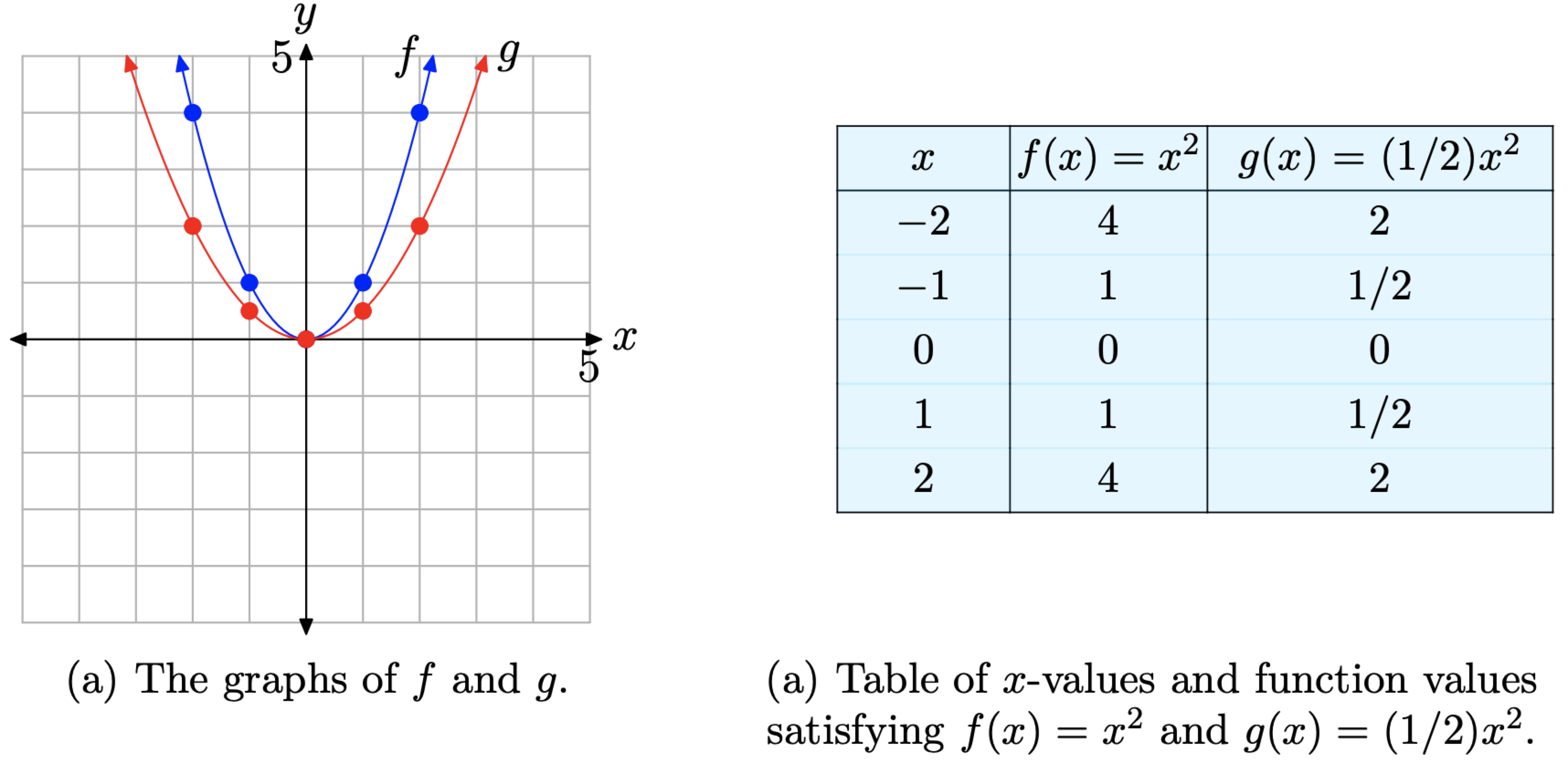
When the points in the table in Figure \(\PageIndex{4}\)(b) are added to the coordinate system in Figure \(\PageIndex{4}\)(a), the resulting graph of g is compressed by a factor of 2 in the vertical direction. It’s as if we again placed the graph of \(f(x) = x^{2}\) on a sheet of rubber graph paper, grabbed the top and bottom of the sheet, and then squeezed them together by a factor of two. Consequently, the graph of \(g(x) = (1/2)x^{2}\) appears somewhat wider in appearance, as seen in comparison to the graph of \(f(x) = x^{2}\) in Figure \(\PageIndex{4}\)(a). Note again that the vertex at the origin is unaffected by this scaling.
If a is a constant smaller than 1 (but larger than zero), that is, if \(0 < a < 1\), then the graph of \(g(x) = ax^{2}\), when compared with the graph of \(f(x) = x^{2}\), is compressed by a factor of 1/a.
Some find Property 4 somewhat counterintuitive. However, if you compare the function \(g(x) = (1/2)x^2\) with the general form \(g(x) = ax^2\), you see that a = 1/2. Property 4 states that the graph will be compressed by a factor of 1/a. In this case, a = 1/2 and
\[\frac{1}{a}=\frac{1}{1 / 2}=2 \nonumber \]
Thus, Property 4 states that the graph of \(g(x) = (1/2)x^2\) should be compressed by a factor of 1/(1/2) or 2, which is seen to be the case in Figure \(\PageIndex{4}\)(a).
Compare the graphs of \(y=x^{2}, y=(1 / 2) x^{2},\) and \(y=(1 / 3) x^{2}\) on your graphing calculator.
Solution
Load the equations \(y=x^{2}, y=(1 / 2) x^{2},\) and \(y=(1 / 3) x^{2}\) into the Y=, as shown in Figure \(\PageIndex{5}\)(a). Push the ZOOM button and select 6:ZStandard to produce the image shown in Figure \(\PageIndex{5}\)(b).
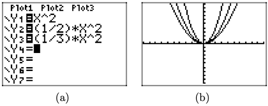
Note that as the “a” in \(y = ax^2\) decreases from 1 to 1/2 to 1/3, the graph of \(y = ax^2\) compresses further and becomes, in a sense, wider in appearance.
Vertical Reflections
Let’s consider the graph of \(g(x) = ax^2\), when a < 0. For example, consider the graphs of \(g(x)=-x^{2}\) and \(h(x)=(-1 / 2) x^{2}\) in Figure \(\PageIndex{6}\)
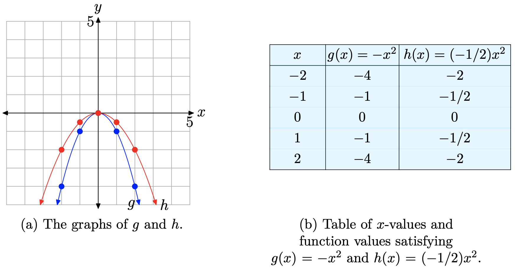
When the table in Figure \(\PageIndex{6}\)(b) is compared with the table in Figure \(\PageIndex{4}\)(b), it is easy to see that the numbers in the last two columns are the same, but they’ve been negated. The result is easy to see in Figure \(\PageIndex{6}\)(a). The graphs have been reflected across the x-axis. Each of the parabolas now “opens downward.”
However, it is encouraging to see that the scaling role of the constant a in \(g(x) = ax^2\) has not changed. In the case of \(h(x) = (−1/2)x^2\), the y-values are still “compressed” by a factor of two, but the minus sign negates these values, causing the graph to reflect across the x-axis. Thus, for example, one would think that the graph of \(y = −2x^2\) would be stretched by a factor of two, then reflected across the x-axis. Indeed, this is correct, and this discussion leads to the following property.
If \(−1 < a < 0\), then the graph of \(g(x) = ax^2\), when compared with the graph of \(f(x) = x^2\), is compressed by a factor of 1/|a|, then reflected across the x-axis. Secondly, if a < −1, then the graph of \(g(x) = ax^2\), when compared with the graph of \(f(x) = x^2\), is stretched by a factor of |a|, then reflected across the x-axis.
Again, some find Property 6 confusing. However, if you compare \(g(x) = (−1/2)x^2\) with the general form \(g(x) = ax^2\), you see that a = −1/2. Note that in this case, −1 < a < 0. Property 6 states that the graph will be compressed by a factor of 1/|a|. In this case, a = −1/2 and
\[\frac{1}{|a|}=\frac{1}{|-1 / 2|}=2 \nonumber \]
That is, Property 6 states that the graph of \(g(x) = (−1/2)x^2\) is compressed by a factor of 1/(| − 1/2|), or 2, then reflected across the x-axis, which is seen to be the case in Figure \(\PageIndex{6}\)(a). Note again that the vertex at the origin is unaffected by this scaling and reflection.
Sketch the graphs of \(y=-2 x^{2}, y=-x^{2},\) and \(y=(-1 / 2) x^{2}\) on your graphing calculator
Solution
Each of the equations were loaded separately into Y1 in the Y= menu. In each of the images in Figure \(\PageIndex{7}\), we selected 6:ZStandard from the ZOOM menu to produce the image.

In Figure \(\PageIndex{7}\)(b), the graph of \(y = −x^2\) is a reflection of the graph of \(y = x^2\) across the x-axis and opens downward. In Figure \(\PageIndex{7}\)(a), note that the graph of \(y = −2x^2\) is stretched vertically by a factor of 2 (compare with the graph of \(y = −x^2\) in Figure \(\PageIndex{7}\)(b)) and reflected across the x-axis to open downward. In Figure \(\PageIndex{7}\)(c), the graph of \((−1/2)x^2\) is compressed by a factor of 2, appears a bit wider, and is reflected across the x-axis to open downward.
Horizontal Translations
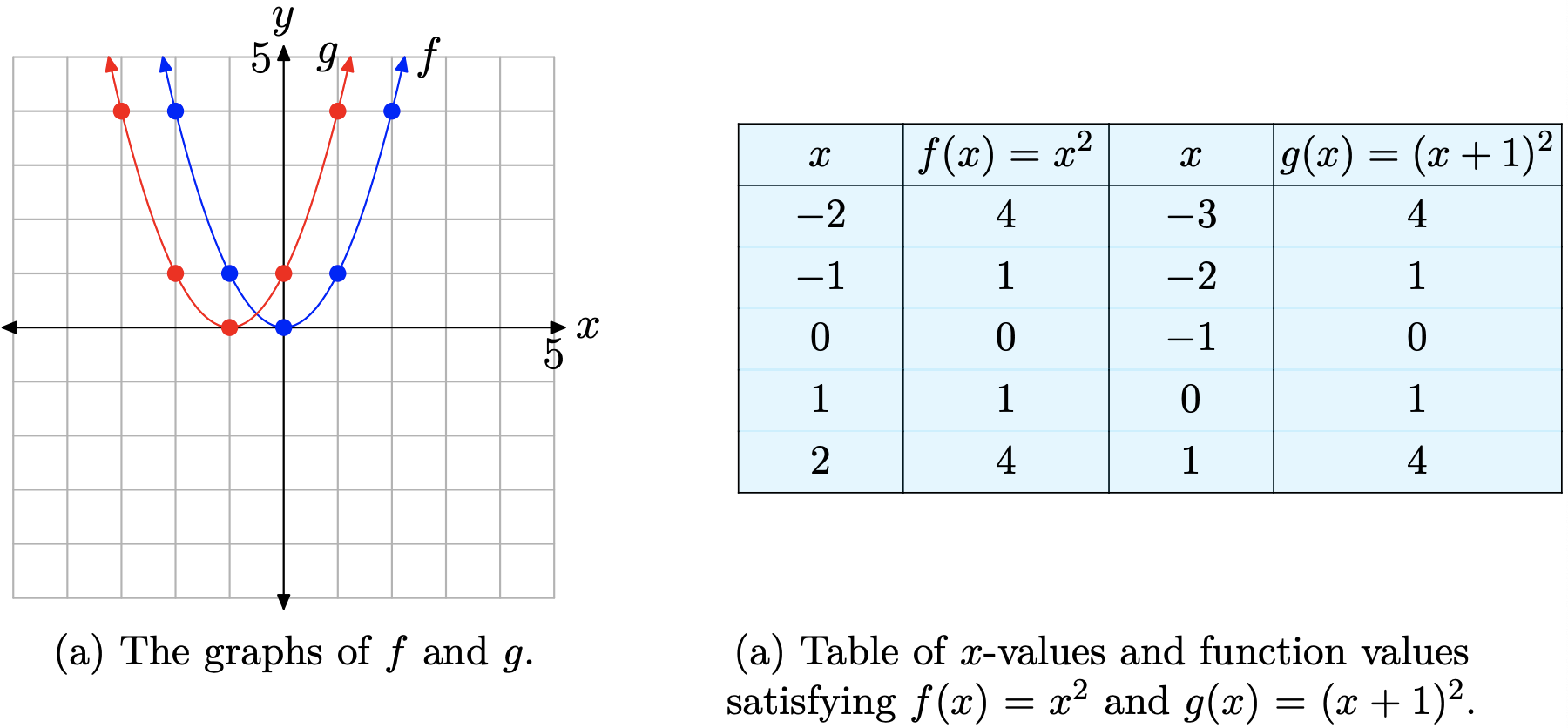
The graph of \(g(x) = (x + 1)^2\) in Figure \(\PageIndex{8}\)(a) shows a basic parabola that is shifted one unit to the left. Examine the table in Figure \(\PageIndex{8}\)(b) and note that the equation \(g(x) = (x + 1)^2\) produces the same y-values as does the equation \(f(x) = x^2\), the only difference being that these y-values are calculated at x-values that are one unit less than those used for \(f(x) = x^2\). Consequently, the graph of \(g(x) = (x + 1)^2\) must shift one unit to the left of the graph of \(f(x) = x^2\), as is evidenced in Figure \(\PageIndex{8}\)(a).
Note that this result is counterintuitive. One would think that replacing x with x + 1 would shift the graph one unit to the right, but the shift actually occurs in the opposite direction.
Finally, note that this time the vertex of the parabola has shifted 1 unit to the left and is now located at the point (−1, 0).
We are led to the following conclusion.
If c > 0, then the graph of \(g(x) = (x + c)^2\) is shifted c units to the left of the graph of \(f(x) = x^2\).
A similar thing happens when you replace x with x − 1, only this time the graph is shifted one unit to the right.
Sketch the graphs of \(y=x^{2}\) and \(y=(x-1)^{2}\) on your graphing calculator.
Solution
Load the equations \(y = x^2\) and \(y = (x − 1)^2\) into the Y= menu, as shown in Figure \(\PageIndex{9}\)(a). Push the ZOOM button and select 6:ZStandard to produce the image shown in Figure \(\PageIndex{9}\)(b).
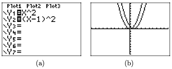
Note that the graph of \(y = (x − 1)^2\) is shifted 1 unit to the right of the graph of \(y = x^2\) and the vertex of the graph of \(y = (x − 1)^2\) is now located at the point (1, 0).
We are led to the following property.
If c > 0, then the graph of \(g(x) = (x − c)^2\) is shifted c units to the right of the graph of \(f(x) = x^2\).
Vertical Translations
The graph of \(g(x) = x^2 + 1\) in Figure \(\PageIndex{10}\)(a) is shifted one unit upward from the graph of \(f(x) = x^2\). This is easy to see as both equations use the same x-values in the table in Figure \(\PageIndex{10}\)(b), but the function values of \(g(x) = x^2 + 1\) are one unit larger than the corresponding function values of \(f(x) = x^2\).
Note that the vertex of the graph of \(g(x) = x^2 + 1\) has also shifted upward 1 unit and is now located at the point (0, 1).
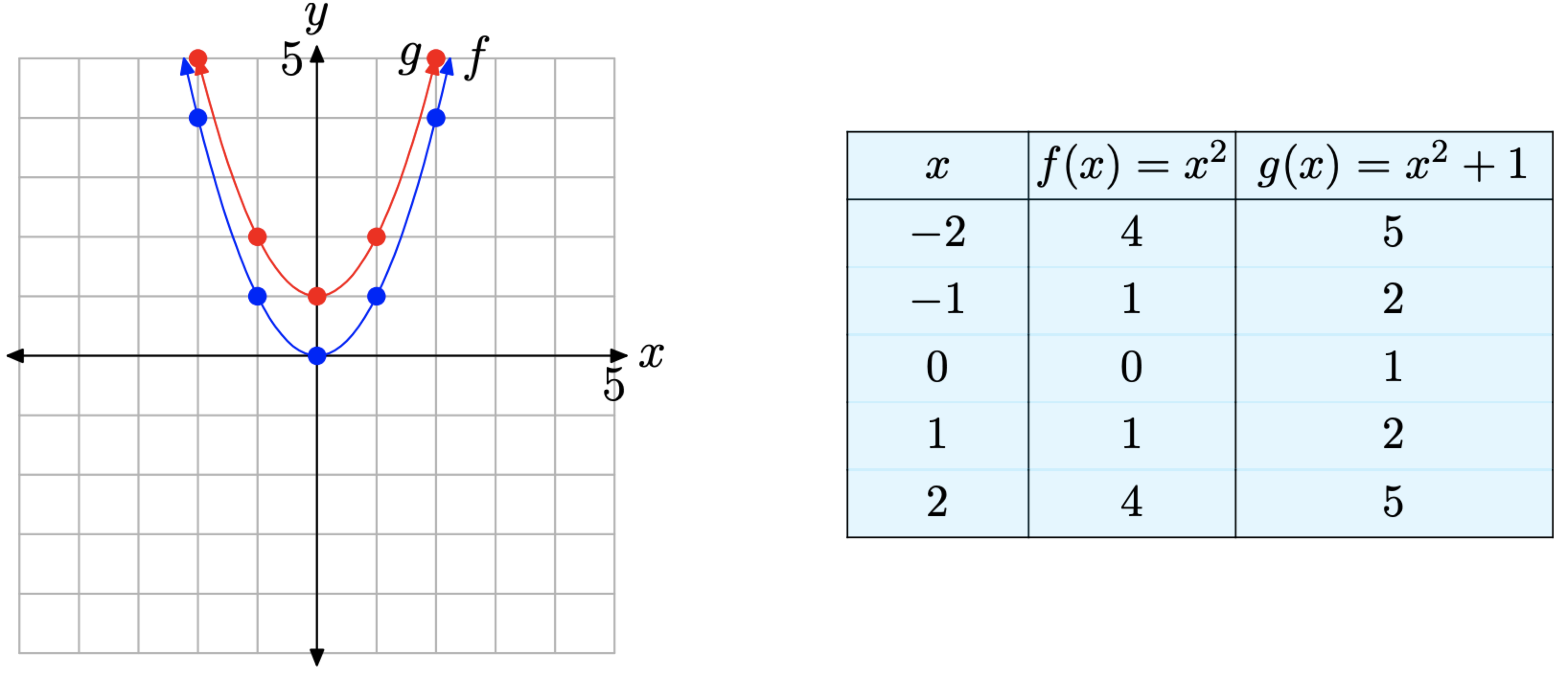
The above discussion leads to the following property.
If c > 0, the graph of \(g(x) = x^2 + c\) is shifted c units upward from the graph of \(f(x) = x^2\).
In a similar vein, the graph of \(y = x^2 − 1\) is shifted downward one unit from the graph of \(y = x^2\)
Sketch the graphs of \(y = x^2\) and \(y = x^2 − 1\) on your graphing calculator.
Solution
Load the equations \(y = x^2\) and \(y = x^2 − 1\) into the Y= menu, as shown in Figure \(\PageIndex{11}\)(a). Push the ZOOM button and select 6:ZStandard to produce the image shown in Figure \(\PageIndex{11}\)(b).
Note that the graph of \(y = x^2 − 1\) is shifted 1 unit downward from the graph of \(y = x^2\) and the vertex of the graph of \(y = x^2 − 1\) is now at the point (0, −1).
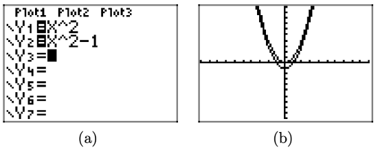
The above discussion leads to the following property.
If c > 0, the graph of \(g(x) = x^2 − c\) is shifted c units downward from the graph of \(f(x) = x^2\).
The Axis of Symmetry
In Figure \(\PageIndex{1}\), the graph of \(y = x^2\) is symmetric with respect to the y-axis. One half of the parabola is a mirror image of the other with respect to the y-axis. We say the y-axis is acting as the axis of symmetry.
If the parabola is reflected across the x-axis, as in Figure 6, the axis of symmetry doesn’t change. The graph is still symmetric with respect to the y-axis. Similar comments are in order for scalings and vertical translations. However, if the graph of \(y = x^2\) is shifted right or left, then the axis of symmetry will change.
Sketch the graph of \(y = −(x + 2)^2 + 3\).
Solution
Although not required, this example is much simpler if you perform reflections before translations.
Tip 15. If at all possible, perform scalings and reflections before translations.
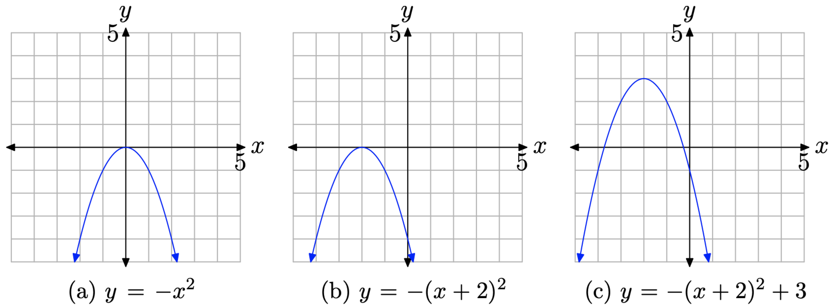
In the series shown in Figure \(\PageIndex{12}\), we first perform a reflection, then a horizontal translation, followed by a vertical translation.
- In Figure \(\PageIndex{12}\)(a), the graph of \(y = −x^2\) is a reflection of the graph of \(y = x^2\) across the x-axis and opens downward. Note that the vertex is still at the origin.
- In Figure \(\PageIndex{12}\)(b), we’ve replaced x with x+ 2 in the equation \(y = −x^2\) to obtain the equation \(y = −(x+ 2)^2\). The effect is to shift the graph of \(y = −x^2\) in Figure \(\PageIndex{12}\)(a) 2 units to the left to obtain the graph of \(y = −(x+ 2)^2\) in Figure \(\PageIndex{12}\)(b). Note that the vertex is now at the point (−2, 0).
- In Figure \(\PageIndex{12}\)(c), we’ve added 3 to the equation \(y = −(x+ 2)^2\) to obtain the equation \(y = −(x+ 2)^2 + 3\). The effect is to shift the graph of y = −(x+ 2)2 in Figure \(\PageIndex{12}\)(b) upward 3 units to obtain the graph of \(y=-(x+2)^{2}+3\) in Figure \(\PageIndex{12}\)(c). Note that the vertex is now at the point (−2, 3).
In practice, we can proceed more quickly. Analyze the equation \(y=-(x+2)^{2}+3\). The minus sign tells us that the parabola “opens downward.” The presence of x + 2 indicates a shift of 2 units to the left. Finally, adding the 3 will shift the graph 3 units upward. Thus, we have a parabola that “opens downward” with vertex at (−2, 3). This is shown in Figure \(\PageIndex{13}\).
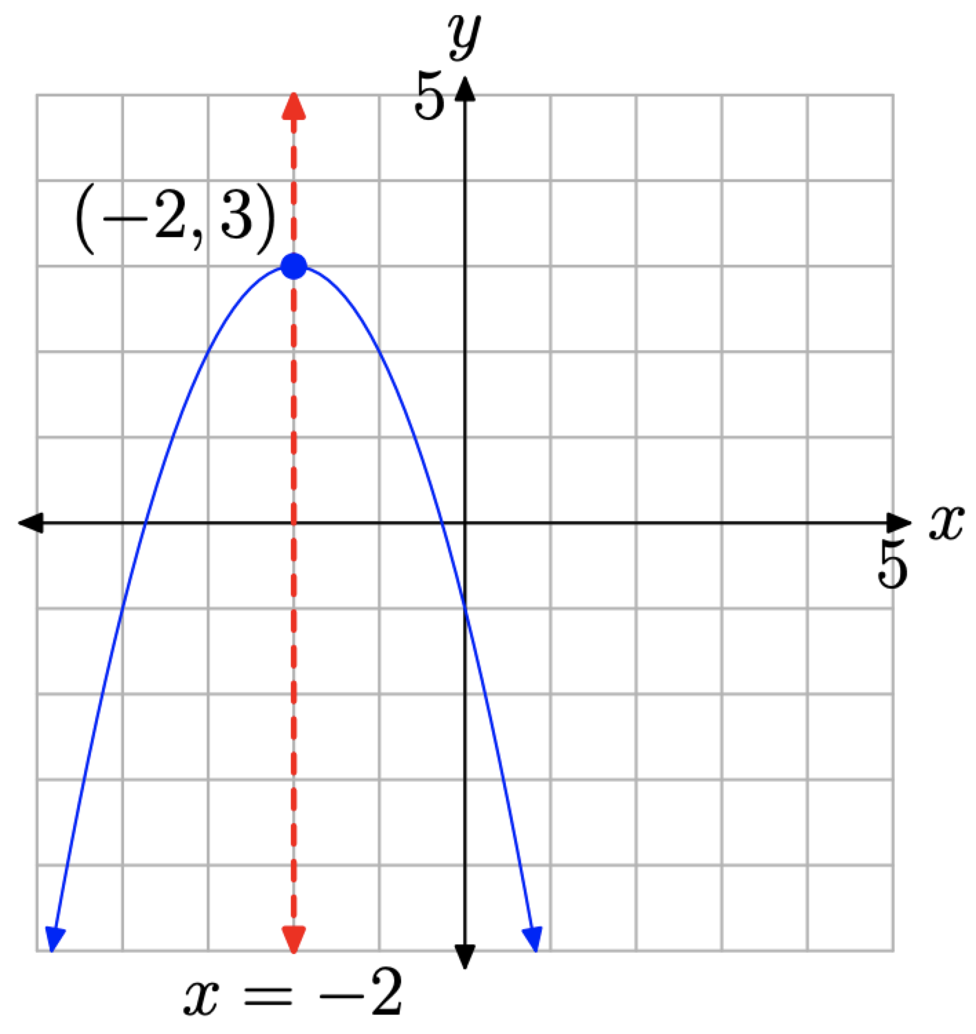
The axis of symmetry passes through the vertex (−2, 3) in Figure \(\PageIndex{13}\) and has equation x = −2. Note that the right half of the parabola is a mirror image of its left half across this axis of symmetry. We can use the axis of symmetry to gain an accurate plot of the parabola with minimal plotting of points.
- Start by plotting the vertex and axis of symmetry as shown in Figure \(\PageIndex{14}\)(a).
- Next, compute two points on either side of the axis of symmetry. We choose x = −1 and x = 0 and compute the corresponding y-values using the equation \(y=-(x+2)^{2}+3\)
| x | \(y=-(x+2)^{2}+3\) |
|---|---|
| -1 | 2 |
| 0 | -1 |
Plot the points from the table, as shown in Figure \(\PageIndex{14}\)(b).
- Finally, plot the mirror images of these points across the axis of symmetry, as shown in Figure \(\PageIndex{14}\)(c).
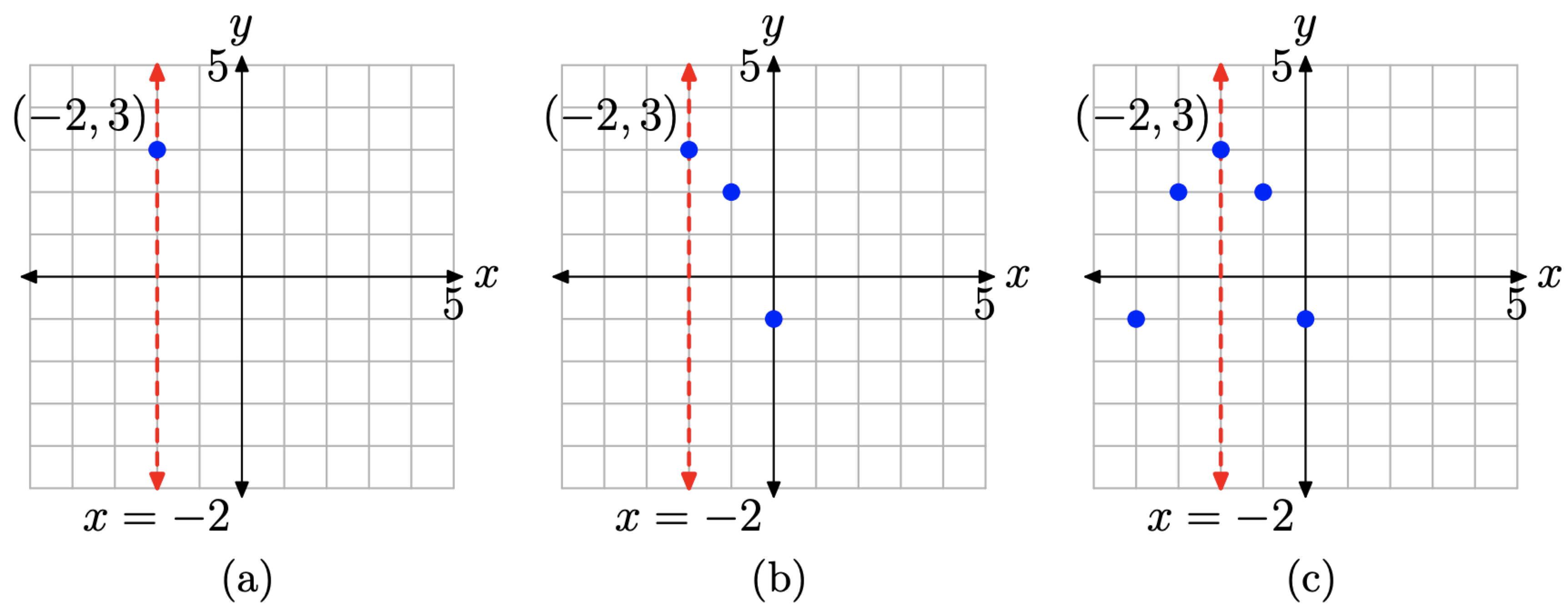
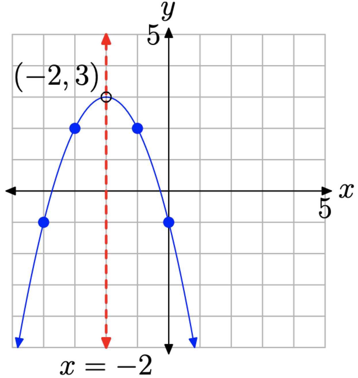
The image in Figure \(\PageIndex{14}\)(c) clearly contains enough information to complete the graph of the parabola having equation \(y=-(x+2)^{2}+3\) in Figure \(\PageIndex{15}\).
Let’s summarize what we’ve seen thus far.
The form of the quadratic function \[f(x)=a(x-h)^{2}+k \nonumber \] is called vertex form. The graph of this quadratic function is a parabola.
- The graph of the parabola opens upward if a > 0, downward if a < 0.
- If the magnitude of a is larger than 1, then the graph of the parabola is stretched by a factor of a. If the magnitude of a is smaller than 1, then the graph of the parabola is compressed by a factor of 1/a.
- The parabola is translated h units to the right if h > 0, and h units to the left if h < 0.
- The parabola is translated k units upward if k > 0, and k units downward if k < 0.
- The coordinates of the vertex are (h, k).
- The axis of symmetry is a vertical line through the vertex whose equation is x = h.
Let’s look at one final example
Use the technique of Example \(\PageIndex{6}\) to sketch the graph of \(f(x) = 2(x − 2)^2 − 3\).
Solution
Compare \(f(x) = 2(x − 2)^2 − 3\) with \(f(x)=a(x-h)^{2}+k\) and note that a = 2. Hence, the parabola has been “stretched” by a factor of 2 and opens upward. The presence of x − 2 indicates a shift of 2 units to the right; and subtracting 3 shifts the parabola 3 units downward. Therefore, the vertex will be located at the point (2, −3) and the axis of symmetry will be the vertical line having equation x = 2. This is shown in Figure \(\PageIndex{16}\)(a).
Some prefer a more strict comparison of \(f(x) = 2(x − 2)^2 − 3\) with the general vertex form \(f(x)=a(x-h)^{2}+k\), yielding a = 2, h = 2, and k = −3. This immediately identifies the vertex at (h, k), or (2, −3).
Next, evaluate the function \(f(x) = 2(x − 2)^2 − 3\) at two points lying to the right of the axis of symmetry (or to the left, if you prefer). Because the axis of symmetry is the vertical line x = 2, we choose to evaluate the function at x = 3 and 4.
\[\begin{array}{l}{f(3)=2(3-2)^{2}-3=-1} \\ {f(4)=2(4-2)^{2}-3=5}\end{array} \nonumber \]
This gives us two points to the right of the axis of symmetry, (3, −1) and (4, 5), which we plot in Figure \(\PageIndex{16}\)(b).
Finally, we plot the mirror images of (3, −1) and (4, 5) across the axis of symmetry, which gives us the points (1, −1) and (0, 5), respectively. These are plotted in Figure \(\PageIndex{16}\)(c). We then draw the parabola through these points.
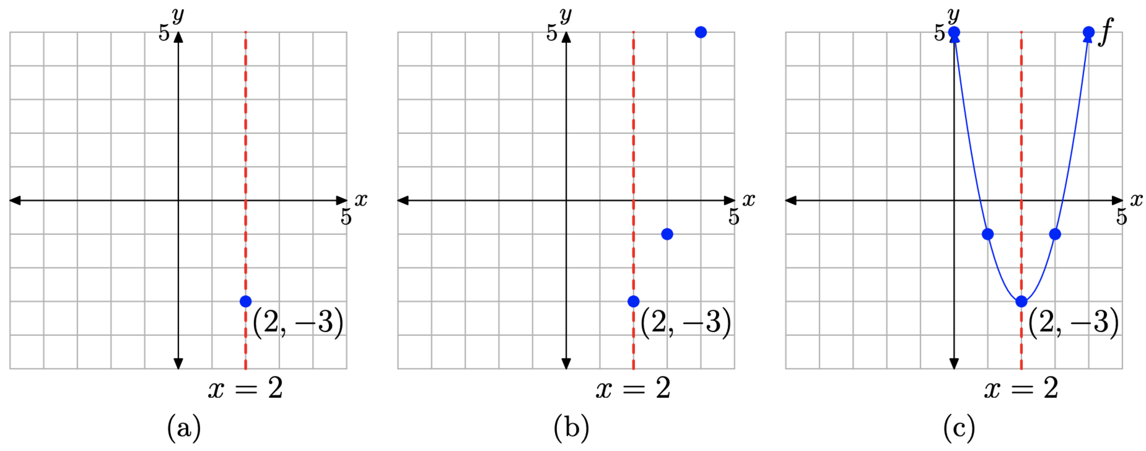
Let’s finish by describing the domain and range of the function defined by the rule \(f(x)=2(x-2)^{2}-3\). If you use the intuitive notion that the domain is the set of “permissible x-values,” then one can substitute any number one wants into the equation \(f(x)=2(x-2)^{2}-3\). Therefore, the domain is all real numbers, which we can write as follows: Domain = \(\mathbb{R}\) or Domain = \((-\infty, \infty)\).
You can also project each point on the graph of \(f(x)=2(x-2)^{2}-3\)onto the x-axis, as shown in Figure \(\PageIndex{17}\)(a). If you do this, then the entire axis will “lie in shadow,” so once again, the domain is all real numbers.
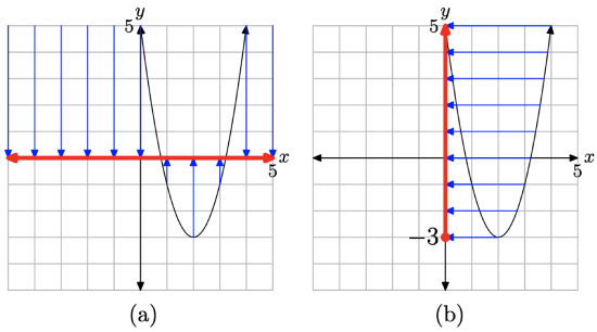
To determine the range of the function \(f(x)=2(x-2)^{2}-3\), project each point on the graph of f onto the y-axis, as shown in Figure \(\PageIndex{17}\)(b). On the y-axis, all points greater than or equal to −3 “lie in shadow,” so the range is described with Range \(=\{y : y \geq-3\}=[-3, \infty)\).
The following summarizes how one finds the domain and range of a quadratic function that is in vertex form.
The domain of the quadratic function \[f(x)=a(x-h)^{2}+k \nonumber \], regardless of the values of the parameters a, h, and k, is the set of all real numbers, easily described with \(\mathbb{R}\) or \((-\infty, \infty)\). On the other hand, the range depends upon the values of a and k.
- If a > 0, then the parabola opens upward and has vertex at (h, k). Consequently, the range will be \[[k, \infty)=\{y : y \geq k\} \nonumber \].
- If a < 0, then the parabola opens downward and has vertex at (h, k). Consequently, the range will be \[(-\infty, k]=\{y : y \leq k\} \nonumber \].
Exercise
In Exercises 1-6, sketch the image of your calculator screen on your homework paper. Label and scale each axis with xmin, xmax, ymin, and ymax. Label each graph with its equation. Remember to use a ruler to draw all lines, including axes.
Use your graphing calculator to sketch the graphs of \(f(x) = x^2\), \(g(x) = 2x^2\), and \(h(x) = 4x^2\) on one screen. Write a short sentence explaining what you learned in this exercise.
- Answer
-
Multiplying by 2 scales vertically by a factor of 2. Multiplying by 4 scales vertically by a factor of 4.
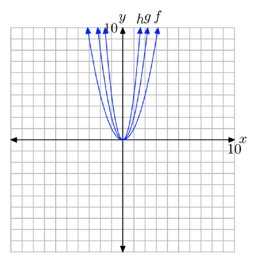
Use your graphing calculator to sketch the graphs of \(f(x) = −x^2\), \(g(x) = −2x^2\), and \(h(x) = −4x^2\) on one screen. Write a short sentence explaining what you learned in this exercise.
Use your graphing calculator to sketch the graphs of \(f(x) = x^2\), \(g(x) = (x−2)^2\), and \(h(x) = (x−4)^2\) on one screen. Write a short sentence explaining what you learned in this exercise.
- Answer
-
The graph of \(g(x) = (x−2)^2\) is shifted 2 units to the right of \(f(x) = x^2\). The graph of \(h(x) = (x−4)^2\) is shifted 4 units to the right of \(f(x) = x^2\).
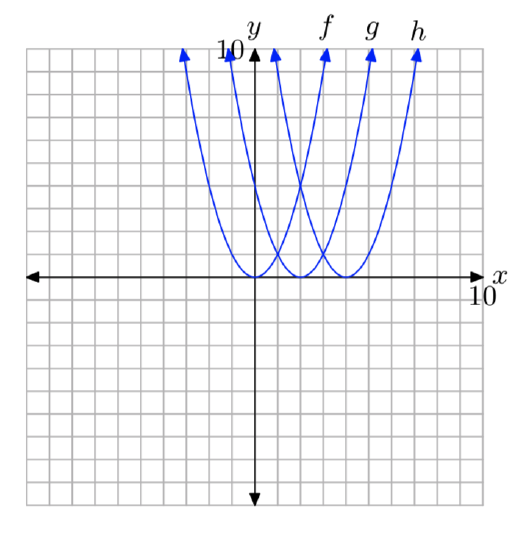
Use your graphing calculator to sketch the graphs of \(f(x) = x^2\), \(g(x) = (x+2)^2\), and \(h(x) = (x+4)^2\) on one screen. Write a short sentence explaining what you learned in this exercise.
Use your graphing calculator to sketch the graphs of \(f(x) = x^2\), \(g(x) = x^2+2\), and \(h(x) = x^2+4\) on one screen. Write a short sentence explaining what you learned in this exercise.
- Answer
-
The graph of \(g(x) = x^2+2\) is shifted 2 units to the upward from the graph of \(f(x) = x^2\).The graph of \(h(x) = x^2+4\) is shifted 4 units upward from the graph of \(f(x) = x^2\).
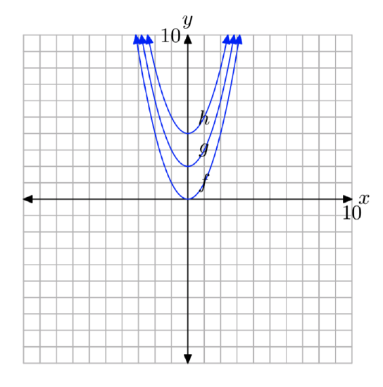
Use your graphing calculator to sketch the graphs of \(f(x) = x^2\), \(g(x) = x^2−2\), and \(h(x) = x^2−4\) on one screen. Write a short sentence explaining what you learned in this exercise.
In Exercises 7-14, write down the given quadratic function on your homework paper, then state the coordinates of the vertex.
\(f(x) = −5(x−4)^2−5\)
- Answer
-
(4, −5)
\(f(x) = 5(x+3)^2−7\)
\(f(x) = 3(x+1)^2\)
- Answer
-
(−1, 0)
\(f(x) = \frac{7}{5}(x+\frac{5}{9})^2−\frac{3}{4}\)
\(f(x) = −7(x−4)^2+6\)
- Answer
-
(4, 6)
\(f(x) = −\frac{1}{2}(x−\frac{8}{9})^2+\frac{2}{9}\)
\(f(x) = \frac{1}{6}(x+\frac{7}{3})^2+\frac{3}{8}\)
- Answer
-
\((−\frac{7}{3}, \frac{3}{8})\)
\(f(x) = −\frac{3}{2}(x+\frac{1}{2})^2−\frac{8}{9}\)
In Exercises 15-22, state the equation of the axis of symmetry of the graph of the given quadratic function.
\(f(x) = −7(x−3)^2+1\)
- Answer
-
x = 3
\(f(x) = −6(x+8)^2+1\)
\(f(x) = −\frac{7}{8}(x+\frac{1}{4})^2+\frac{2}{3}\)
- Answer
-
\(x = −\frac{1}{4}\)
\(f(x) = −\frac{1}{2}(x−\frac{3}{8})^2−\frac{5}{7}\)
\(f(x) = −\frac{2}{9}(x+\frac{2}{3})^2−\frac{4}{5}\)
- Answer
-
\(x = −\frac{2}{3}\)
\(f(x) = −7(x+3)^2+9\)
\(f(x) = −\frac{8}{7}(x+\frac{2}{9})^2+\frac{6}{5}\)
- Answer
-
\(x = −\frac{2}{9}\)
\(f(x) = 3(x+3)^2+6\)
In Exercises 23-36, perform each of the following tasks for the given quadratic function.
- Set up a coordinate system on graph paper. Label and scale each axis.
- Plot the vertex of the parabola and label it with its coordinates.
- Draw the axis of symmetry and label it with its equation.
- Set up a table near your coordinate system that contains exact coordinates of two points on either side of the axis of symmetry. Plot them on your coordinate system and their “mirror images” across the axis of symmetry.
- Sketch the parabola and label it with its equation.
- Use interval notation to describe both the domain and range of the quadratic function.
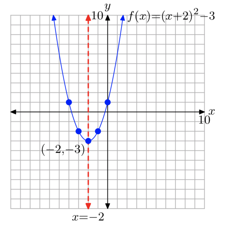
\(f(x) = (x+2)^2−3\)
- Answer
-
Domain= \((−\infty, \infty)\); Range= [−3, \(\infty\))
\(f(x) = (x−3)^2−4\)
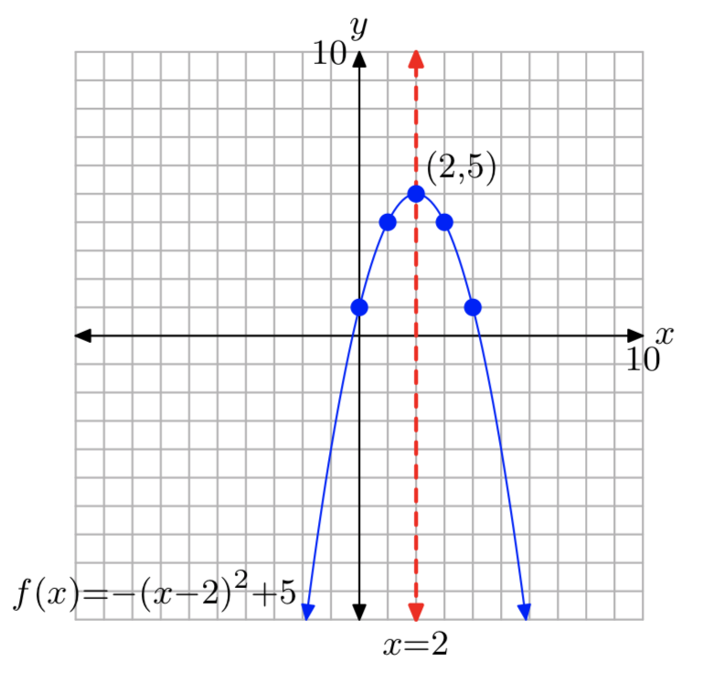
\(f(x) = −(x−2)^2+5\)
- Answer
-
Domain= \((−\infty, \infty)\); Range= (−\(\infty\), 5]
\(f(x) = −(x+4)^2+4\)
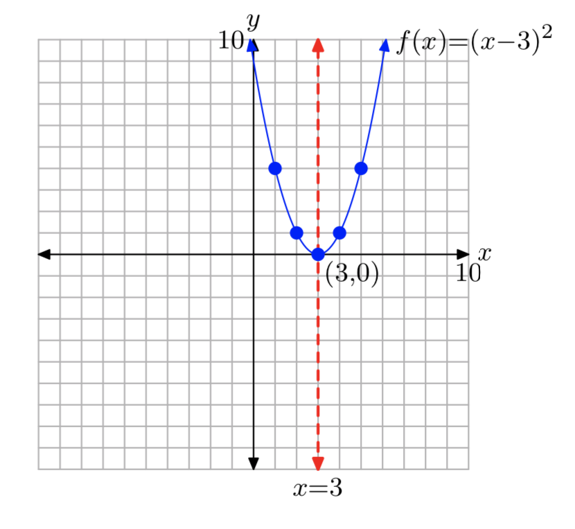
\(f(x) = (x−3)^2\)
- Answer
-
Domain= \((−\infty, \infty)\); Range= [0, \(\infty\))
\(f(x) = −(x+2)^2\)
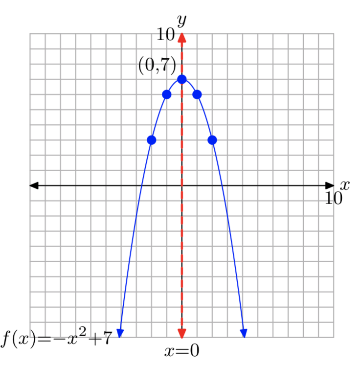
\(f(x) = −x^2+7\)
- Answer
-
Domain= \((−\infty, \infty)\); Range= (−\(\infty\), 7]
\(f(x) = −x^2+7\)
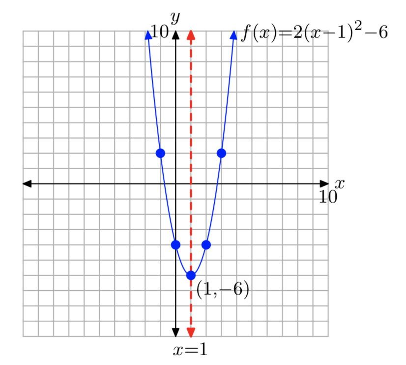
\(f(x) = 2(x−1)^2−6\)
- Answer
-
Domain= \((−\infty, \infty)\); Range= [−6, \(\infty\))
\(f(x) = −2(x+1)^2+5\)
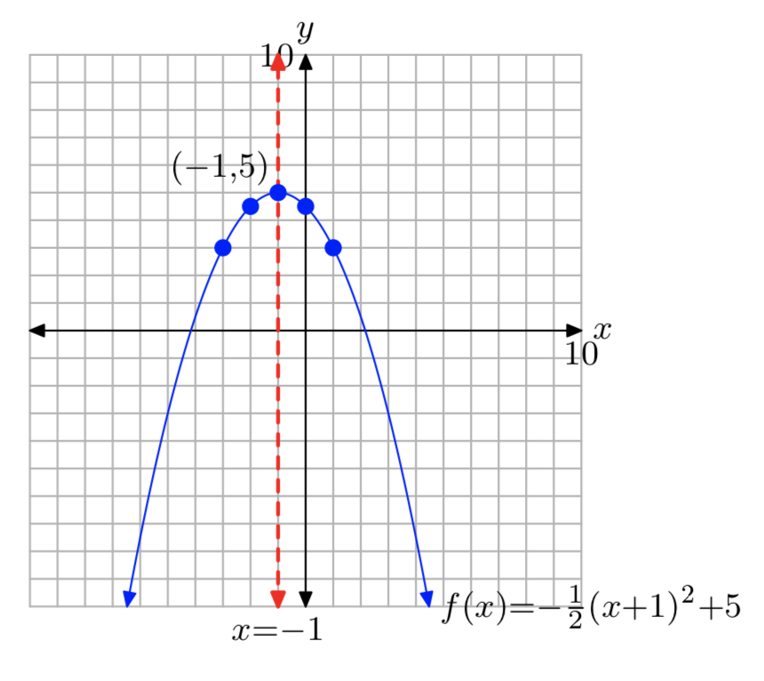
\(f(x) = −\frac{1}{2}(x+1)^2+5\)
- Answer
-
Domain= \((−\infty, \infty)\); Range= (−\(\infty\), 5]
\(f(x) = \frac{1}{2}(x−3)^2−6\)
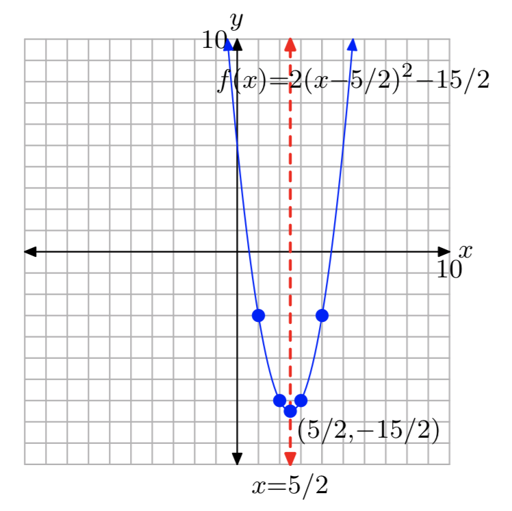
\(f(x) = 2(x−\frac{5}{2})^2−\frac{15}{2}\)
- Answer
-
Domain= \((−\infty, \infty)\); Range= [−\(\frac{15}{2}\), \(\infty\))
\(f(x) = −3(x+\frac{7}{2})^2+\frac{15}{4}\)
In Exercises 37-44, write the given quadratic function on your homework paper, then use set-builder and interval notation to describe the domain and the range of the function.
\(f(x) = 7(x+6)^2−6\)
- Answer
-
Domain= \((−\infty, \infty)\); Range = [−6, \(\infty\)) = {y: \(y \ge −6\)}
\(f(x) = 8(x+1)^2+7\)
\(f(x) = −3(x+4)^2−7\)
- Answer
-
Domain= \((−\infty, \infty)\); Range = (−\(\infty\), −7] = {y: \(y \le −7\)}
\(f(x) = −6(x−7)^2+9\)
\(f(x) = −7(x+5)^2−7\)
- Answer
-
Domain= \((−\infty, \infty)\); Range = (−\(\infty\), −7] = {y: \(y \le −7\)}
\(f(x) = 8(x−4)^2+3\)
\(f(x) = −4(x−1)^2+2\)
- Answer
-
Domain= \((−\infty, \infty)\); Range = (−\(\infty\), 2] = {y: \(y \le 2\)}
\(f(x) = 7(x−2)^2−3\)
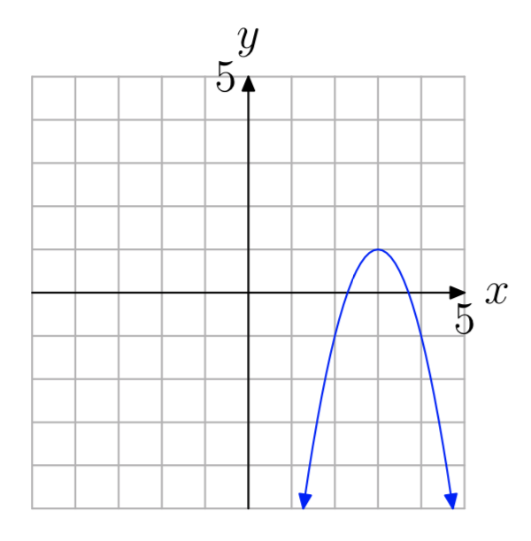
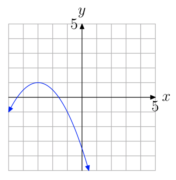
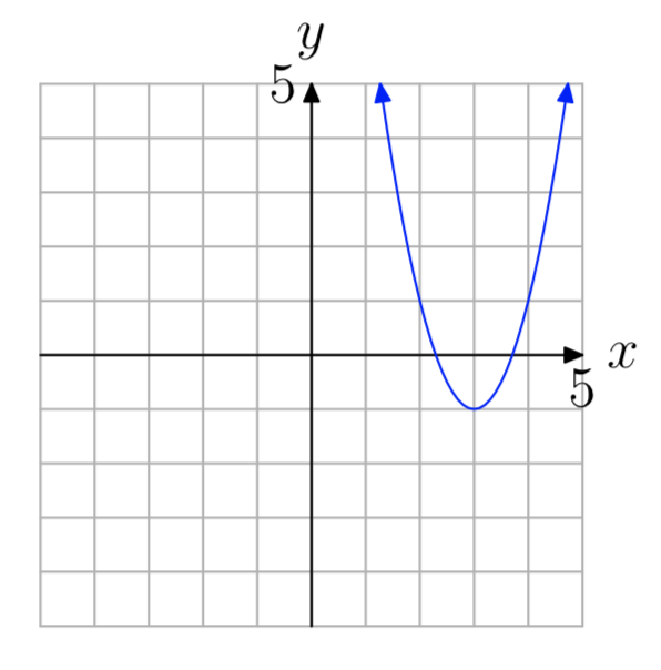
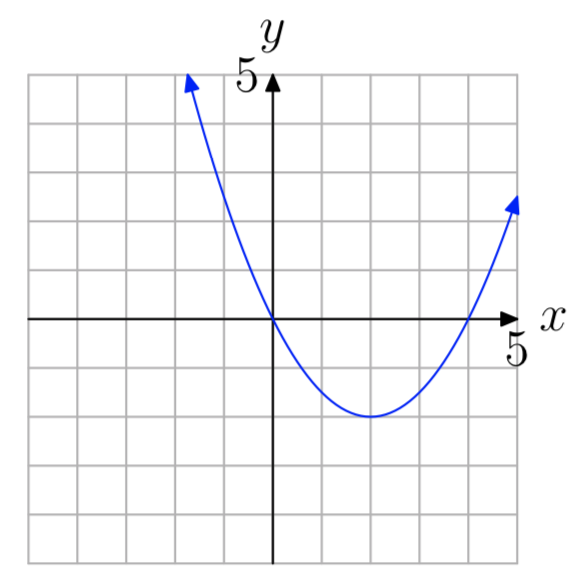
In Exercises 45-52, using the given value of a, find the specific quadratic function of the form \(f(x) = a(x−h)^2+k\) that has the graph shown. Note: h and k are integers. Check your solution with your graphing calculator.
a = −2
- Answer
-
\(f(x) = −2(x−3)^2+1\)
a = 0.5
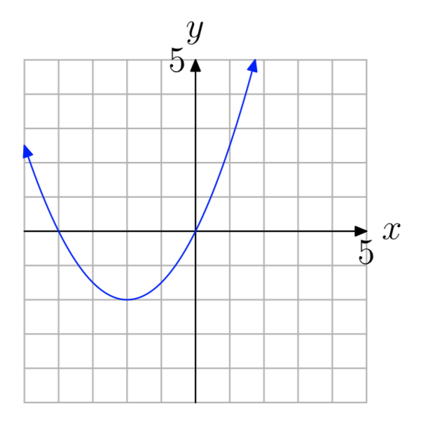
a = 2
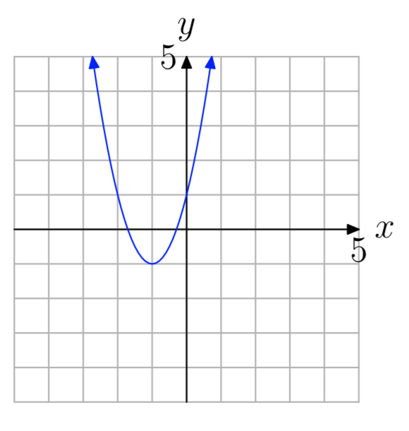
- Answer
-
\(f(x) = 2(x+1)^2−1\)
a = 0.5
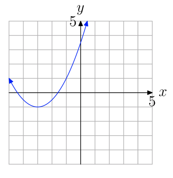
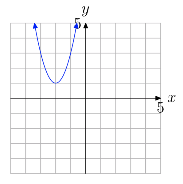
- Answer
-
\(f(x) = 2(x+2)^2+1\)
a = −0.5
a = 2
- Answer
-
\(f(x) = 2(x−3)^2−1\)
a = 0.5
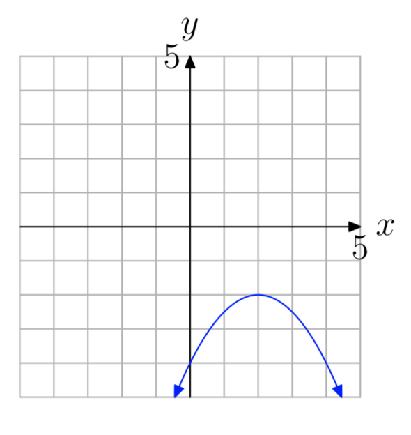
In Exercises 53-54, use the graph to determine the range of the function \(f(x) = ax^2+bx+c\) The arrows on the graph are meant to indicate that the graph continues indefinitely in the continuing pattern and direction of each arrow. Describe your solution using interval notation.
- Answer
-
(\(−\infty\), −2]
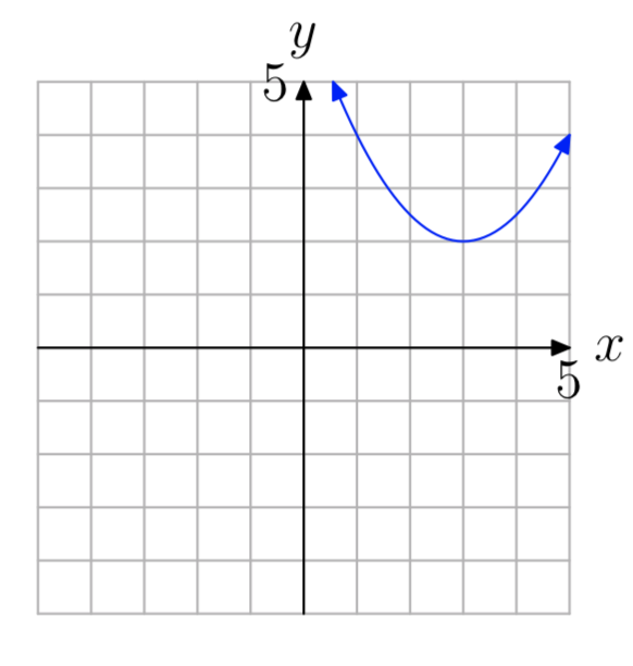
In Exercises 55-56, use the graph to determine the domain of the function \(f(x) = ax^2+bx+c\). The arrows on the graph are meant to indicate that the graph continues indefinitely in the continuing pattern and direction of each arrow. Use interval notation to describe your solution.
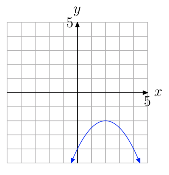
- Answer
-
\((−\infty, \infty)\)
