8.2: Exponential Functions
- Page ID
- 19728

\( \newcommand{\vecs}[1]{\overset { \scriptstyle \rightharpoonup} {\mathbf{#1}} } \)
\( \newcommand{\vecd}[1]{\overset{-\!-\!\rightharpoonup}{\vphantom{a}\smash {#1}}} \)
\( \newcommand{\dsum}{\displaystyle\sum\limits} \)
\( \newcommand{\dint}{\displaystyle\int\limits} \)
\( \newcommand{\dlim}{\displaystyle\lim\limits} \)
\( \newcommand{\id}{\mathrm{id}}\) \( \newcommand{\Span}{\mathrm{span}}\)
( \newcommand{\kernel}{\mathrm{null}\,}\) \( \newcommand{\range}{\mathrm{range}\,}\)
\( \newcommand{\RealPart}{\mathrm{Re}}\) \( \newcommand{\ImaginaryPart}{\mathrm{Im}}\)
\( \newcommand{\Argument}{\mathrm{Arg}}\) \( \newcommand{\norm}[1]{\| #1 \|}\)
\( \newcommand{\inner}[2]{\langle #1, #2 \rangle}\)
\( \newcommand{\Span}{\mathrm{span}}\)
\( \newcommand{\id}{\mathrm{id}}\)
\( \newcommand{\Span}{\mathrm{span}}\)
\( \newcommand{\kernel}{\mathrm{null}\,}\)
\( \newcommand{\range}{\mathrm{range}\,}\)
\( \newcommand{\RealPart}{\mathrm{Re}}\)
\( \newcommand{\ImaginaryPart}{\mathrm{Im}}\)
\( \newcommand{\Argument}{\mathrm{Arg}}\)
\( \newcommand{\norm}[1]{\| #1 \|}\)
\( \newcommand{\inner}[2]{\langle #1, #2 \rangle}\)
\( \newcommand{\Span}{\mathrm{span}}\) \( \newcommand{\AA}{\unicode[.8,0]{x212B}}\)
\( \newcommand{\vectorA}[1]{\vec{#1}} % arrow\)
\( \newcommand{\vectorAt}[1]{\vec{\text{#1}}} % arrow\)
\( \newcommand{\vectorB}[1]{\overset { \scriptstyle \rightharpoonup} {\mathbf{#1}} } \)
\( \newcommand{\vectorC}[1]{\textbf{#1}} \)
\( \newcommand{\vectorD}[1]{\overrightarrow{#1}} \)
\( \newcommand{\vectorDt}[1]{\overrightarrow{\text{#1}}} \)
\( \newcommand{\vectE}[1]{\overset{-\!-\!\rightharpoonup}{\vphantom{a}\smash{\mathbf {#1}}}} \)
\( \newcommand{\vecs}[1]{\overset { \scriptstyle \rightharpoonup} {\mathbf{#1}} } \)
\(\newcommand{\longvect}{\overrightarrow}\)
\( \newcommand{\vecd}[1]{\overset{-\!-\!\rightharpoonup}{\vphantom{a}\smash {#1}}} \)
\(\newcommand{\avec}{\mathbf a}\) \(\newcommand{\bvec}{\mathbf b}\) \(\newcommand{\cvec}{\mathbf c}\) \(\newcommand{\dvec}{\mathbf d}\) \(\newcommand{\dtil}{\widetilde{\mathbf d}}\) \(\newcommand{\evec}{\mathbf e}\) \(\newcommand{\fvec}{\mathbf f}\) \(\newcommand{\nvec}{\mathbf n}\) \(\newcommand{\pvec}{\mathbf p}\) \(\newcommand{\qvec}{\mathbf q}\) \(\newcommand{\svec}{\mathbf s}\) \(\newcommand{\tvec}{\mathbf t}\) \(\newcommand{\uvec}{\mathbf u}\) \(\newcommand{\vvec}{\mathbf v}\) \(\newcommand{\wvec}{\mathbf w}\) \(\newcommand{\xvec}{\mathbf x}\) \(\newcommand{\yvec}{\mathbf y}\) \(\newcommand{\zvec}{\mathbf z}\) \(\newcommand{\rvec}{\mathbf r}\) \(\newcommand{\mvec}{\mathbf m}\) \(\newcommand{\zerovec}{\mathbf 0}\) \(\newcommand{\onevec}{\mathbf 1}\) \(\newcommand{\real}{\mathbb R}\) \(\newcommand{\twovec}[2]{\left[\begin{array}{r}#1 \\ #2 \end{array}\right]}\) \(\newcommand{\ctwovec}[2]{\left[\begin{array}{c}#1 \\ #2 \end{array}\right]}\) \(\newcommand{\threevec}[3]{\left[\begin{array}{r}#1 \\ #2 \\ #3 \end{array}\right]}\) \(\newcommand{\cthreevec}[3]{\left[\begin{array}{c}#1 \\ #2 \\ #3 \end{array}\right]}\) \(\newcommand{\fourvec}[4]{\left[\begin{array}{r}#1 \\ #2 \\ #3 \\ #4 \end{array}\right]}\) \(\newcommand{\cfourvec}[4]{\left[\begin{array}{c}#1 \\ #2 \\ #3 \\ #4 \end{array}\right]}\) \(\newcommand{\fivevec}[5]{\left[\begin{array}{r}#1 \\ #2 \\ #3 \\ #4 \\ #5 \\ \end{array}\right]}\) \(\newcommand{\cfivevec}[5]{\left[\begin{array}{c}#1 \\ #2 \\ #3 \\ #4 \\ #5 \\ \end{array}\right]}\) \(\newcommand{\mattwo}[4]{\left[\begin{array}{rr}#1 \amp #2 \\ #3 \amp #4 \\ \end{array}\right]}\) \(\newcommand{\laspan}[1]{\text{Span}\{#1\}}\) \(\newcommand{\bcal}{\cal B}\) \(\newcommand{\ccal}{\cal C}\) \(\newcommand{\scal}{\cal S}\) \(\newcommand{\wcal}{\cal W}\) \(\newcommand{\ecal}{\cal E}\) \(\newcommand{\coords}[2]{\left\{#1\right\}_{#2}}\) \(\newcommand{\gray}[1]{\color{gray}{#1}}\) \(\newcommand{\lgray}[1]{\color{lightgray}{#1}}\) \(\newcommand{\rank}{\operatorname{rank}}\) \(\newcommand{\row}{\text{Row}}\) \(\newcommand{\col}{\text{Col}}\) \(\renewcommand{\row}{\text{Row}}\) \(\newcommand{\nul}{\text{Nul}}\) \(\newcommand{\var}{\text{Var}}\) \(\newcommand{\corr}{\text{corr}}\) \(\newcommand{\len}[1]{\left|#1\right|}\) \(\newcommand{\bbar}{\overline{\bvec}}\) \(\newcommand{\bhat}{\widehat{\bvec}}\) \(\newcommand{\bperp}{\bvec^\perp}\) \(\newcommand{\xhat}{\widehat{\xvec}}\) \(\newcommand{\vhat}{\widehat{\vvec}}\) \(\newcommand{\uhat}{\widehat{\uvec}}\) \(\newcommand{\what}{\widehat{\wvec}}\) \(\newcommand{\Sighat}{\widehat{\Sigma}}\) \(\newcommand{\lt}{<}\) \(\newcommand{\gt}{>}\) \(\newcommand{\amp}{&}\) \(\definecolor{fillinmathshade}{gray}{0.9}\)Let’s suppose that the current population of the city of Pleasantville is 10000 and that the population is growing at a rate of 2% per year. In order to analyze the population growth over a period of years, we’ll try to develop a formula for the population as a function of time, and then graph the result.
First, note that at the end of one year, the population increase is 2% of 10000, or 200 people. We would now have 10,200 people in Pleasantville. At the end of the second year, take another 2% of 10200, which is an increase of 204 people, for a total of 10404. Because the increase each year is not constant, the graph of population versus time cannot be a line. Hence, our eventual population function will not be linear.
To develop our population formula, we start by letting the function P(t) represent the population of Pleasantville at time t, where we measure t in years. We will start time at t = 0 when the initial population of Pleasantville is 10000. In other words, P(0) = 10000. The key to understanding this example is the fact that the population increases by 2% each year. We are making an assumption here that this overall growth accounts for births, deaths, and people coming into and leaving Pleasantville. That is, at the end of the first year, the population of Pleasantville will be 102% of the initial population. Thus,
\[P(1) = 1.02P(0) = 1.02(10000). \label{1} \]
We could multiply out the right side of this equation, but it will actually be more useful to leave it in its current form.
Now each year the population increases by 2%. Therefore, at the end of the second year, the population will be 102% of the population at the end of the first year. In other words,
\[P(2) = 1.02P(1). \label{2} \]
If we replace \(P(1)\) in Equation \ref{2} with the result found in Equation \ref{1}, then
\[P(2) = (1.02)(1.02)(10000) = (1.02)^{2}(10000). \label{3} \]
Let’s iterate one more year. At the end of the third year, the population will be 102% of the population at the end of the second year, so
\[P(3) = 1.02P(2). \label{4} \]
However, if we replace \(P(2)\) in Equation \ref{4} with the result found in Equation \ref{3}, we obtain
\[P(3) = (1.02)(1.02)^{2}(10000) = (1.02)^{3}(10000). \label{5} \]
The pattern should now be clear. The population at the end of \(t\) years is given by the function.
\[P(t) = (1.02)^{t}(10000) \nonumber \]
It is traditional in mathematics and science to place the initial population in front in this formula, writing instead
\[P(t) = 10000(1.02)^{t}. \label{6} \]
Our function \(P(t)\) is defined by Equation \ref{6} for all positive integers {1, 2, 3, . . .}, and \(P(0) = 10000\), the initial population. Figure 1 shows a plot of our function. Although points are plotted only at integer values of t from 0 to 40, that’s enough to show the trend of the population over time. The population starts at 10000, increases over time, and the yearly increase (the difference in population from one year to the next) also gets larger as time passes.
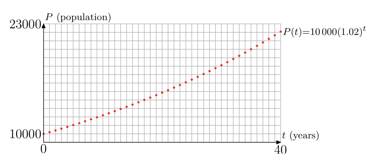
We can now use the function P(t) to predict the population in later years. Assuming that the growth rate of 2% continues, what will the population of Pleasantville be after 40 years? What will it be after 100 years?
Solution
Substitute \(t = 40\) and \(t = 100\) into Equation \ref{6}. The population in 40 years will be
\[P(40) = 10000(1.02)^{40} \approx 22080 \nonumber \]
and the population in 100 years will be
\[P(100) = 10000(1.02)^{100} \approx 72446. \nonumber \]
What would be different if we had started with a population of 12000? By tracing over our previous steps, it should be easy to see that the new formula would be
\[P(t) = 12000(1.02)^{t}. \nonumber \]
Similarly, if the growth rate had been 3% per year instead of 2%, then we would have ended up with the formula
\[P(t) = 10000(1.03)^t. \nonumber \]
Thus, by letting \(P_{0}\) represent the initial population, and \(r\) represent the growth rate (in decimal form), we can generalize the formula to
\[P(t) = P_{0}(1+r)^{t}. \label{8)} \]
Note that our formula for the function \(P(t)\) is different from the previous functions that we’ve studied so far, in that the input variable \(t\) is part of the exponent in the formula. Thus, this is a new type of function.
Now let’s contrast the situation in Pleasantville with the population dynamics of Ghosttown. Ghosttown also starts with a population of 10000, but several factories have closed, so some people are leaving for better opportunities. In this case, the population of Ghosttown is decreasing at a rate of 2% per year. We’ll again develop a formula for the population as a function of time, and then graph the result.
First, note that at the end of one year, the population decrease is 2% of 10000, or 200 people. We would now have 9800 people left in Ghosttown. At the end of the second year, take another 2% of 9800, which is a decrease of 196 people, for a total of 9604. As before, because the decrease each year is not constant, the graph of population versus time cannot be a line, so our eventual population function will not be linear.
Now let the function \(P(t)\) represent the population of Ghosttown at time \(t\), where we measure \(t\) in years. The initial population of Ghosttown at \(t = 0\) is 10000, so \(P(0) = 10,000\). Since the population decreases by 2% each year, at the end of the first year the population of Ghosttown will be 98% of the initial population. Thus,
\[P(1) = 0.98P(0) = 0.98(10000). \label{9} \]
Each year the population decreases by 2%. Therefore, at the end of the second year, the population will be 98% of the population at the end of the first year. In other words,
\[P(2) = 0.98P(1). \label{10} \]
If we replace \(P (1)\) in Equation \ref{10} with the result found in Equation \ref{9}, then
\[P(2) = (0.98)(0.98)(10 000) = (0.98)^{2}(10000). \label{11} \]
Let’s iterate one more year. At the end of the third year, the population will be 98% of the population at the end of the second year, so
\[P(3) = 0.98P(2). \label{12} \]
However, if we replace \(P (2)\) in Equation \ref{12} with the result found in Equation \label{11}, we obtain
\[P(3) = (0.98)(0.98)^{2}(10000) = (0.98)^{3}(10000). \label{13} \]
The pattern should now be clear. The population at the end of \(t\) years is given by the function
\[P(t) = (0.98)^{t}(10000), \nonumber \]
Or equivalently,
\[P(t) = 10000(0.98)^t\). \label{14} \]
Our function \(P(t)\) is defined by Equation \ref{14} for all positive integers {1, 2, 3, . . .}, and P(0) = 10000, the initial population. Figure 2 shows a plot of our function. Although points are plotted only at integer values of t from 0 to 40, that’s enough to show the trend of the population over time. The population starts at 10 000, decreases over time, and the yearly decrease (the difference in population from one year to the next) also gets smaller as time passes.
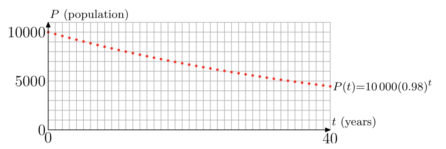
Assuming that the rate of decrease continues at 2%, predict the population of Ghosttown after 40 years and after 100 years.
Solution
Substitute \(t = 40\) and \(t = 100\) into Equation \ref{14}. The population in 40 years will be
\(P(40) = 10000(0.98)^{40} \approx 4457\),
and the population in 100 years will be
\(P(100) = 10000(0.98)^{100} \approx 1326\).
Note that if we had instead started with a population of 9000, for example, then the new formula would be
\(P(t) = 9000(0.98)^t\).
Similarly, if the rate of decrease had been 5% per year instead of 2%, then we would have ended up with the formula
\(P(t) = 10000(0.95)^t\).
Thus, by letting \(P_{0}\) represent the initial population, and \(r\) represent the growth rate (in decimal form), we can generalize the formula to
\[P(t) = P_{0}(1−r)^t. \label{16} \]
Definition
As noted before, our functions \(P(t)\) in our Pleasantville and Ghosttown examples are a new type of function, because the input variable \(t\) is part of the exponent in the formula.
An exponential function is a function of the form
\(f(t) = b^t\)
where b > 0 and \(b \ne 1\). \(b\) is called the base of the exponential function. More generally, a function of the form
\(f(t) = Ab^t\),
where b > 0, \(b \ne 1\), and \(A \ne 0\), is also referred to as an exponential function. In this case, the value of the function when t = 0 is f(0) = A, so A is the initial amount.
In applications, you will almost always encounter exponential functions in the more general form \(Ab^t\). In fact, note that in the previous population examples, the function P(t) has this form \(P(t) = Ab^t\), with \(A = P_{0}\), \(b = 1+r\) in Pleasantville, and \(b = 1−r\) in Ghosttown. In particular, \(A = P_{0}\) is the initial population.
Since exponential functions are often used to model processes that vary with time, we usually use the input variable \(t\) (although of course any variable can be used). Also, you may be curious why the definition says \(b \ne 1\), since \(1^t\) just equals 1. We’ll explain this curiosity at the end of this section.
Graphs of Exponential Functions
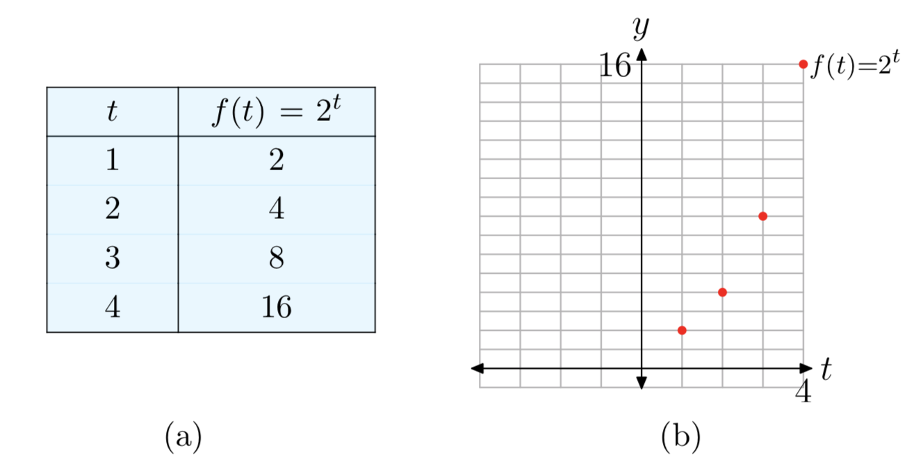
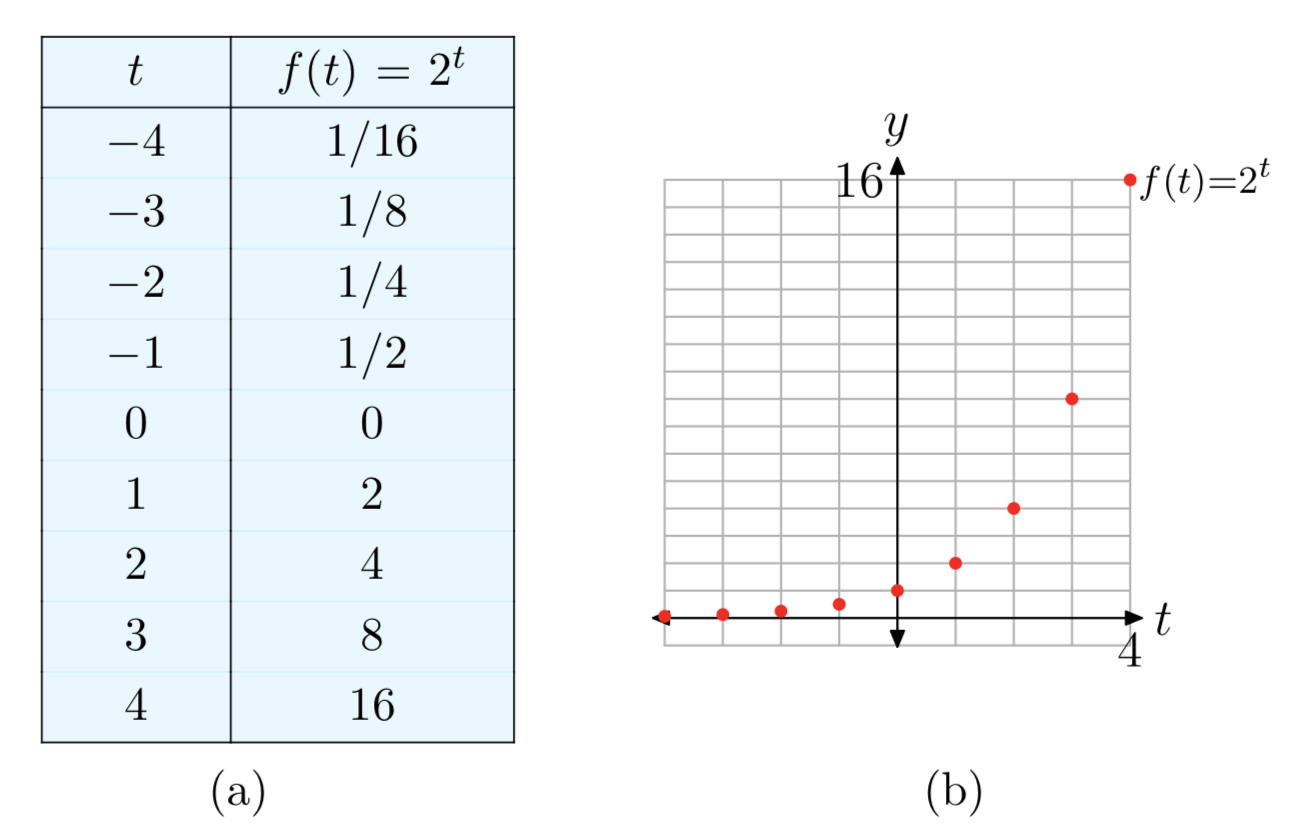
We’ll develop the properties for the basic exponential function \(b^t\) first, and then note the minor changes for the more general form \(Ab^t\). For a working example, let’s use base b = 2, and let’s compute some values of \(f(t) = 2^t\) and plot the result (Figure 3).
Recall from the previous section that 2t is also defined for negative exponents t and the 0 exponent. Thus, the exponential function \(f(t) = 2^t\) is defined for all integers. Figure 4 shows a new table and plot with points added at 0 and negative integer values.
However, the previous section showed that \(2^t\) is also defined for rational and irrational exponents. Therefore, the domain of the exponential function \(f(t) = 2^t\) is the set of all real numbers. When we add in the values of the function at all rational and irrational values of \(t\), we obtain a final continuous curve as shown in Figure 5.
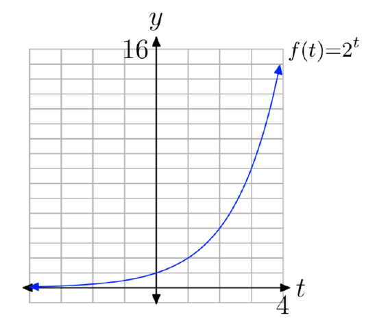
Note several properties of the graph in Figure 5:
- Moving from left to right, the curve rises, which means that the function increases as t increases. In fact, the function increases rapidly for positive t.
- The graph lies above the t-axis, so the values of the function are always positive. Therefore, the range of the function is \((0, \infty)\).
- The graph has a horizontal asymptote y = 0 (the t-axis) on the left side. This means that the function almost “dies out” (the values get closer and closer to 0) as t approaches \(−\infty\).
What about the graphs of other exponential functions with different bases? We’ll use the calculator to explore several of these.
First, use your calculator to compare \(y_{1}(x) = 2^x\) and \(y_{2}(x) = 3^x\). As can be seen in Figure 6(a), the graph of \(3^x\) rises faster that \(2^x\) for x > 0, and dies out faster for x < 0.
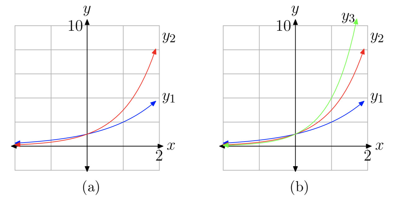
Next, add in \(y_{3}(x) = 4^x\). The result is shown in Figure 6(b). Again, increasing the size of the base to b = 4 results in a function which rises even faster on the right and likewise dies out faster on the left. If you continue to increase the size of the base b, you’ll see that this trend continues. That’s not terribly surprising because, if we compute the value of these functions at a fixed positive x, for example at x = 2, then the values increase: \(2^2 < 3^2 < 4^2 < ....\) Similarly, at x = −2, the values decrease: \(2^{−2} > 3^{−2} > 4^{−2} >....\)
All of the functions in our experiments so far share the properties listed in (a)–(c) above: the function increases, the range is \((0, \infty)\), and the graph has a horizontal asymptote y = 0 on the left side. Now let’s try smaller values of the base b. First use the calculator to plot the graph of \(y_{1}(x) = (\frac{1}{2})^x\) (see Figure 7(a)).
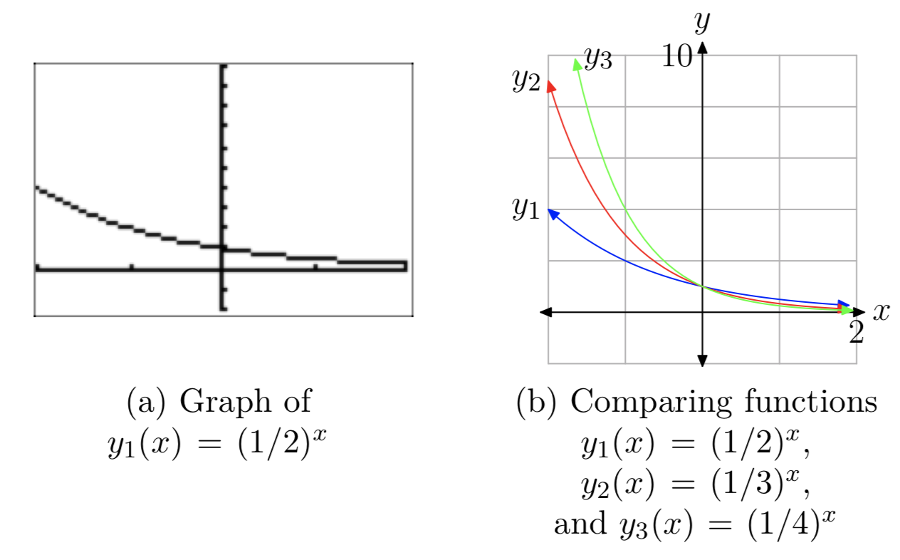
This graph is much different. It rises rapidly to the left, and almost dies out on the right. Compare this with \(y_{2}(x) = (\frac{1}{3})^x\) and \(y_{3}(x) = (\frac{1}{4})^x\) (see Figure 7(b)). As the base gets smaller, the graph rises faster on the left, and dies out faster on the right.
Using reflection properties, it’s easy to understand the appearance of these last three graphs. Note that
\((\frac{1}{2})^x = (2^{−1})^x = 2^{−x}\)
so it follows that the graph of \((\frac{1}{2})^x\) is just a reflection in the y-axis of the graph of \(2^x\) (see Figure 8).
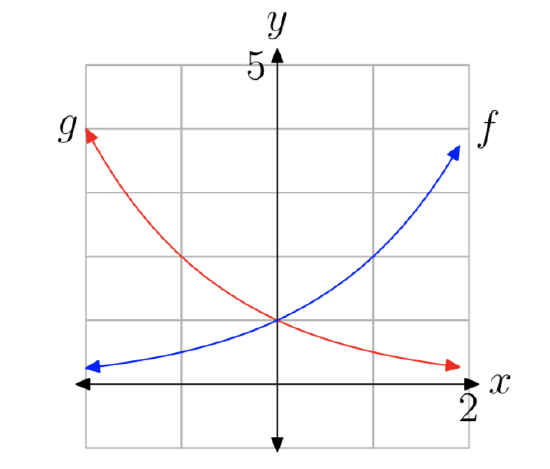
Thus, we seem to have two different types of graphs, and therefore two types of exponential functions: one type is increasing, and the other decreasing. Our experiments above, along with a little more experimentation, should convince you that \(b^x\) is increasing for b > 1, and decreasing for 0 < b < 1. The first type of functions are called exponential growth functions, and the second type are exponential decay functions.
- The domain is the set of all real numbers.
- Moving from left to right, the graph rises, which means that the function increases as x increases. The function increases rapidly for positive x.
- The graph lies above the x-axis, so the values of the function are always positive. Therefore, the range is \((0, \infty)\).
- The graph has a horizontal asymptote y = 0 (the x-axis) on the left side. This means that the function almost “dies out” (the values get closer and closer to 0) as x approaches \(−\infty\).
The second property above deserves some additional explanation. Looking at Figure 6(b), it appears that \(y_{2}\) and \(y_{3}\) increase rapidly as x increases, but \(y_{1}\) appears to increase slowly. However, this is due to the fact that the graph of \(y_{1}(x) = 2^x\) is only shown on the interval [−2, 2]. In Figure 5, the same function is graphed on the interval [−4, 4], and it certainly appears to increase rapidly in that graph. The point here is that exponential growth functions eventually increase rapidly as x increases. If you graph the function on a large enough interval, the function will eventually become very steep on the right side of the graph. This is an important property of the exponential growth functions, and will be explored further in the exercises.
- The domain is the set of all real numbers.
- Moving from left to right, the graph falls, which means that the function de- creases as x increases. The function decreases rapidly for negative x.
- The graph lies above the x-axis, so the values of the function are always positive. Therefore, the range is \((0, \infty)\).
- The graph has a horizontal asymptote y = 0 (the x-axis) on the right side. This means that the function almost “dies out” (the values get closer and closer to 0) as x approaches \(\infty\).
Why do we refrain from using the base b = 1? After all, \(1^x\) is certainly defined: it has the value 1 for all x. But that means that \(f(x) = 1^x\) is just a constant linear function – its graph is a horizontal line. Therefore, this function doesn’t share the same properties as the other exponential functions, and we’ve already classified it as a linear function. Thus, \(1^x\) is not considered to be an exponential function.
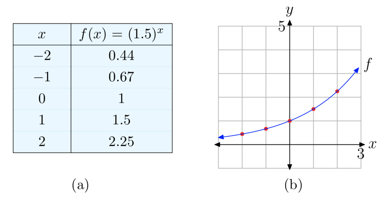
Plot the graph of the function \(f(x) = (1.5)^x\). Identify the range of the function and the horizontal asymptote.
Solution
Since the base 1.5 is larger than 1, this is an exponential growth function. Therefore, its graph will have a shape similar to the graphs in Figure 6. The graph rises, there will be a horizontal asymptote y = 0 on the left side, and the range of the function is \((0, \infty)\). The graph can then be plotted by hand by using this knowledge along with approximate values at x = −2, −1, 0, 1, 2. See Figure 9.
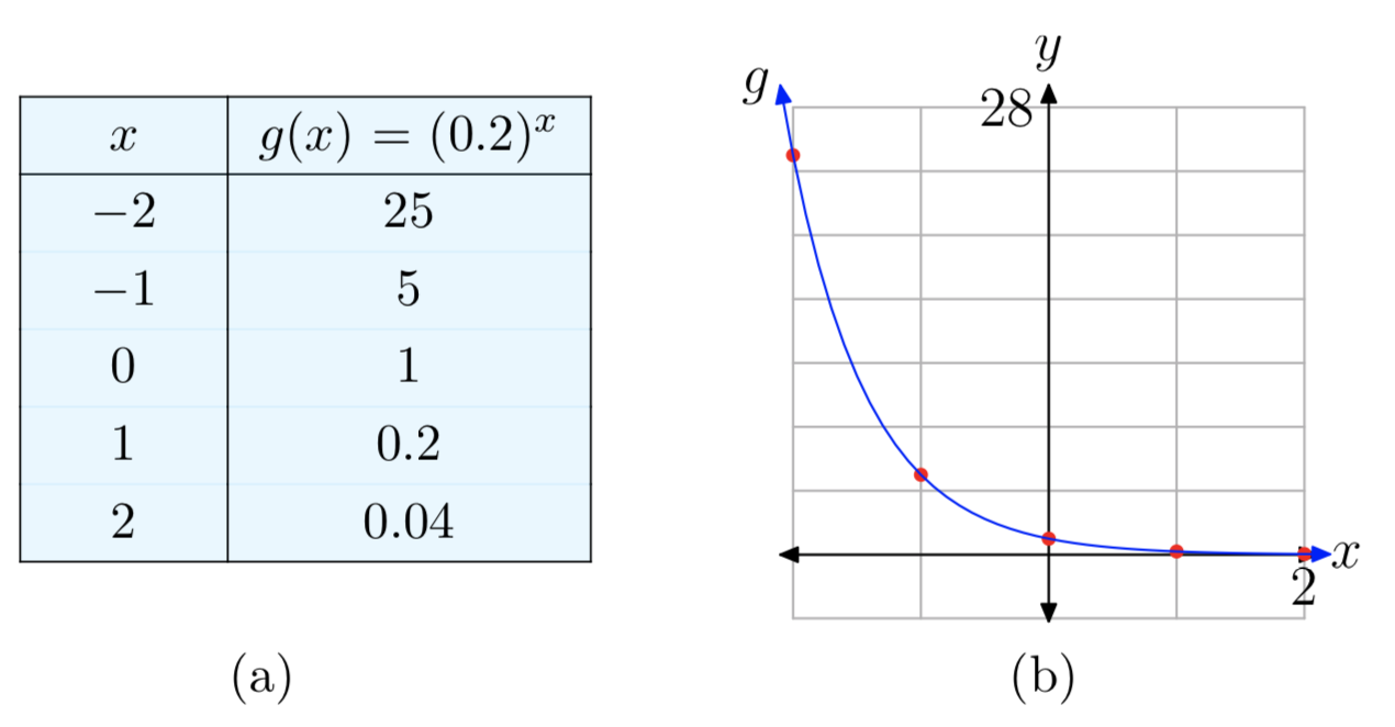
Plot the graph of the function \(g(x) = (0.2)^x\). Identify the range of the function and the horizontal asymptote.
Solution
Since the base 0.2 is smaller than 1, this is an exponential decay function. Therefore, its graph will have a shape similar to the graphs in Figure 7. The graph falls, there will be a horizontal asymptote y = 0 on the right side, and the range of the function is \((0, \infty)\). The graph can then be plotted by hand by using this knowledge along with approximate values at x = −2, −1, 0, 1, 2. See Figure 10.
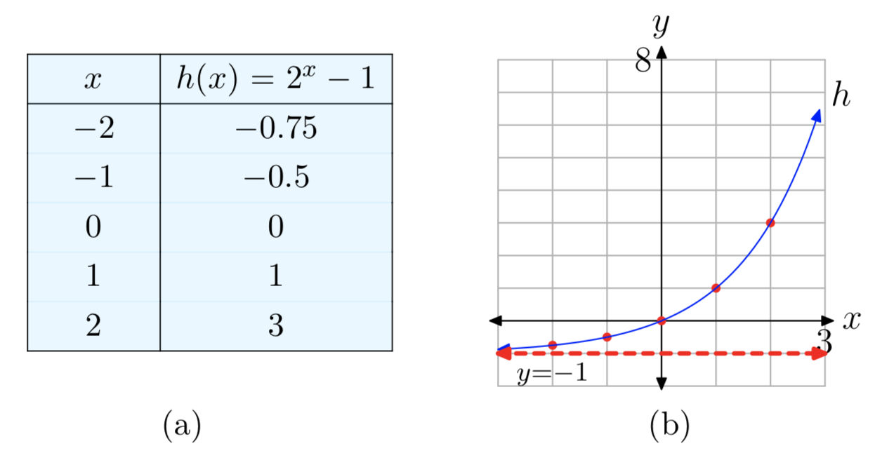
Plot the graph of the function \(f(x) = 2^x−1\). Identify the range of the function and the horizontal asymptote.
Solution
The graph of h can be obtained from the graph of \(f(x) = 2^x\) (see Figure 5) by a vertical shift down 1 unit. Therefore, the horizontal asymptote y = 0 of the graph of f will also be shifted down 1 unit, so the graph of h has a horizontal asymptote y = −1. Similarly, the range of f will be shifted down to \((−1, \infty)\) = Range(h). The graph can then be plotted by hand by using this knowledge along with approximate values at x = −2, −1, 0, 1, 2. See Figure 11.
In later sections of this chapter, we will also see more general exponential functions of the form \(f(x) = Ab^x\) (in fact, the Pleasantville and Ghosttown functions at the beginning of this section are of this form). If A is positive, then the graphs of these functions can be obtained from the basic exponential graphs by vertical scaling, so the graphs will have the same general shape as either the exponential growth curves (if b > 1) or the exponential decay curves (if \(0 < b < 1\)) we plotted earlier.
Exercise
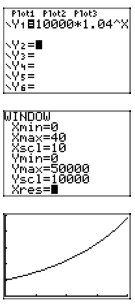
The current population of Fortuna is 10,000 hearty souls. It is known that the population is growing at a rate of 4% per year. Assuming this rate remains constant, perform each of the following tasks.
- Set up an equation that models the population P(t) as a function of time t.
- Use the model in the previous part to predict the population 40 years from now.
- Use your calculator to sketch the graph of the population over the next 40 years.
- Answer
-
- \(P(t) = 10000(1.04)^t\)
- \(P(40) \approx 48101\)
The population of the town of Imagination currently numbers 12,000 people. It is known that the population is growing at a rate of 6% per year. Assuming this rate remains constant, perform each of the following tasks.
- Set up an equation that models the population P(t) as a function of time t.
- Use the model in the previous part to predict the population 30 years from now.
- Use your calculator to sketch the graph of the population over the next 30 years.
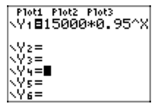
The population of the town of Despairia currently numbers 15,000 individuals. It is known that the population is decaying at a rate of 5% per year. Assuming this rate remains constant, perform each of the following tasks.
- Set up an equation that models the population P(t) as a function of time t.
- Use the model in the previous part to predict the population 50 years from now.
- Use your calculator to sketch the graph of the population over the next 50 years.
- Answer
-
- \(p(t) = 15 000(0.95)^t\)
- \(P(50) \approx 1154\)
The population of the town of Hopeless currently numbers 25,000 individuals. It is known that the population is decaying at a rate of 6% per year. Assuming this rate remains constant, perform each of the following tasks.
- Set up an equation that models the population P(t) as a function of time t.
- Use the model in the previous part to predict the population 40 years from now.
- Use your calculator to sketch the graph of the population over the next 40 years.
In Exercises 5-12, perform each of the following tasks for the given function.
- Find the y-intercept of the graph of the function. Also, use your calculator to find two points on the graph to the right of the y-axis, and two points to the left.
- Using your five points from (a) as a guide, set up a coordinate system on graph paper. Choose and label appropriate scales for each axis. Plot the five points, and any additional points you feel are necessary to discern the shape of the graph.
- Draw the horizontal asymptote with a dashed line, and label it with its equation.
- Sketch the graph of the function.
- Use interval notation to describe both the domain and range of the function.
\(f(x) = (2.5)^x\)
- Answer
-
- The y-intercept is (0, 1). Evaluating the function at x = 1, 2, −1, −2 to obtain the points (1, 2.5), (2, 6.25), (−1, 0.4), (−2, 0.16) (other answers are possible).
- See the graph in part (4).
- The horizontal asymptote is y = 0. See the graph in part (4).
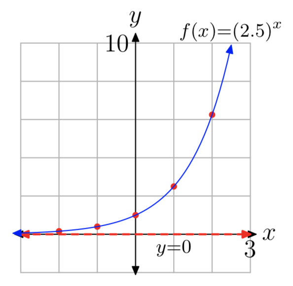
- Domain = \((−\infty, \infty)\), Range = \((0, \infty)\)
\(f(x) = (0.1)^x\)
\(f(x) = (0.75)^x\)
- Answer
-
- The y-intercept is (0, 1). Evaluate the function at x = 1, 2, −1, −2 to obtain the points (1, 0.75), (2, 0.56), (−1, 1.34), (−2, 1.78) (other answers are possible).
- See the graph in part (4).
- The horizontal asymptote is y = 0. See the graph in part (4).
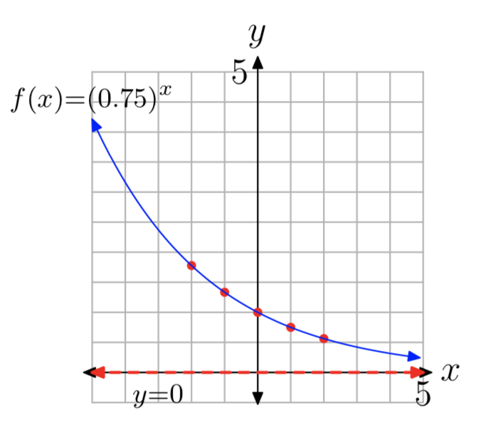
- Domain = \((−\infty, \infty)\), Range = \((0, \infty)\)
\(f(x) = (1.1)^x\)
\(f(x) = 3^x+1\)
- Answer
-
- The y-intercept is (0, 2). Evaluate the function at x = 1, 2, −1, −2 to obtain the points (1, 4), (2, 10), (−1, 1.34), (−2, 1.11) (other answers are possible).
- See the graph in part (4).
- The horizontal asymptote is y = 1. See the graph in part (4).
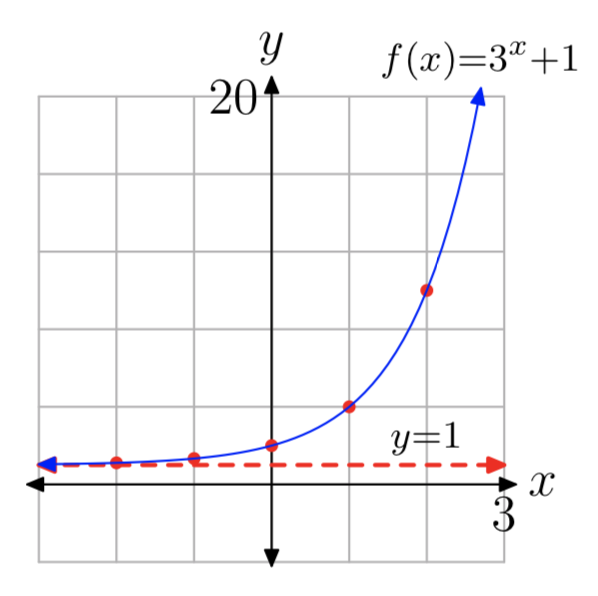
- Domain = \((−\infty, \infty)\), Range = \((1, \infty)\)
\(f(x) = 4^x−5\)
\(f(x) = 2^x−3\)
- Answer
-
- The y-intercept is (0, −2). Evaluate the function at x = 1, 2, −1, −2 to obtain the points (1, −1), (2, 1), (−1, −2.5), (−2, −2.75) (other answers are possible).
- See the graph in part (4).
- The horizontal asymptote is y = −3. See the graph in part (4).
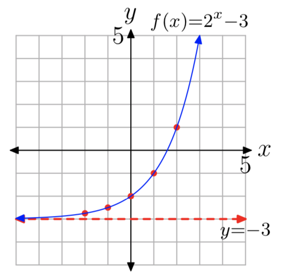
- Domain = \((−\infty, \infty)\), Range = \((−3, \infty)\)
\(f(x) = 5^x+2\)
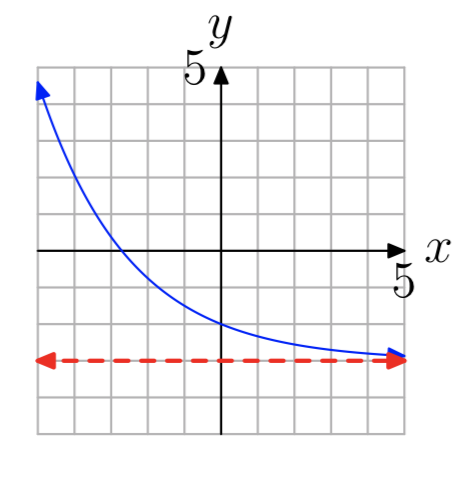
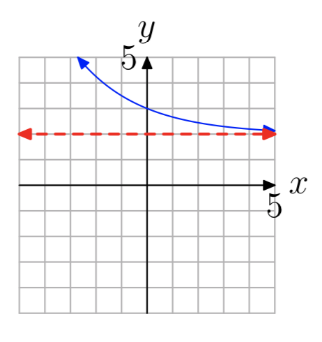
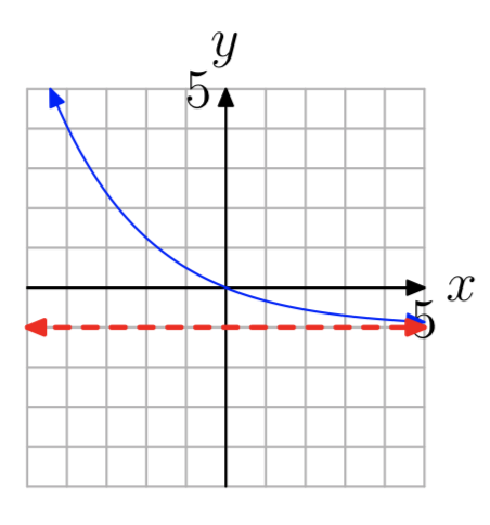
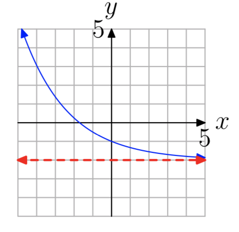
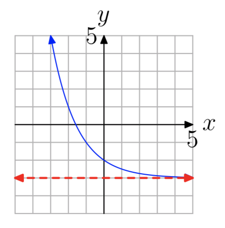
In Exercises 13-20, the graph of an exponential function of the form \(f(x) = b^x+c\) is shown. The dashed red line is a horizontal asymptote. Determine the range of the function. Express your answer in interval notation.
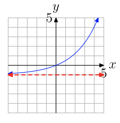
- Answer
-
\((−1, \infty)\)
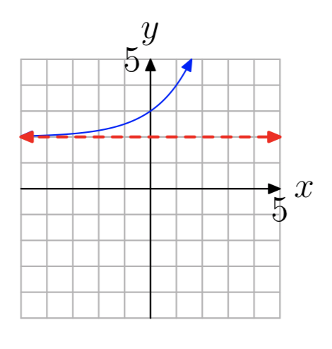
- Answer
-
\((2, \infty)\)
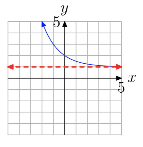
- Answer
-
\((2, \infty)\)
- Answer
-
\((−2, \infty)\)
In Exercises 21-32, compute f(p) at the given value p.
\(f(x) = (\frac{1}{3})^x\); p = −4
- Answer
-
81
\(f(x) = (\frac{3}{4})^x\); p = 1
\(f(x) = 5^x\); p = 5
- Answer
-
3125
\(f(x) = (\frac{1}{3})^x\); p = 4
\(f(x) = 4^x\); p = −4
- Answer
-
\(\frac{1}{256}\)
\(f(x) = 5^x\); p = −3
\(f(x) = (\frac{5}{2})^x\); p = −3
- Answer
-
\(\frac{8}{125}\)
\(f(x) = 9^x\); p = 3
\(f(x) = 5^x\); p = −4
- Answer
-
\(\frac{1}{625}\)
\(f(x) = 9^x\); p = 0
\(f(x) = (\frac{6}{5})^x\); p = −4
- Answer
-
\(\frac{625}{1296}\)
\(f(x) = (\frac{3}{5})^x\); p = 0
In Exercises 33-40, use your calculator to evaluate the function at the given value p. Round your answer to the nearest hundredth.
\(f(x) = 10^x\); p = −0.7.
- Answer
-
0.20
\(f(x) = 10^x\); p = −1.6.
\(f(x) = (\frac{2}{5})^x\); p = 3.67.
- Answer
-
0.03
\(f(x) = 2^x\); \(p = −\frac{3}{4}\).
\(f(x) = 10^x\); p = 2.07.
- Answer
-
117.49
\(f(x) = 7^x\); \(p = \frac{4}{3}\).
\(f(x) = 10^x\); \(p = −\frac{1}{5}\).
- Answer
-
0.63
\(f(x) = (\frac{4}{3})^x\); p = 1.15
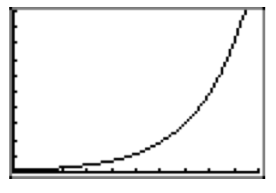
This exercise explores the property that exponential growth functions eventually increase rapidly as x increases. Let \(f(x) = 1.05^x\). Use your graphing calculator to graph f on the intervals
(a) [0, 10] and (b) [0, 100].
For (a), use Ymin = 0 and Ymax = 10.
For (b), use Ymin = 0 and Ymax = 100.
Make accurate copies of the images in your viewing window on your homework paper. What do you observe when you compare the two graphs?
- Answer
-
(a) The graph on the interval [0, 10] increases very slowly. In fact, the graph looks almost linear.
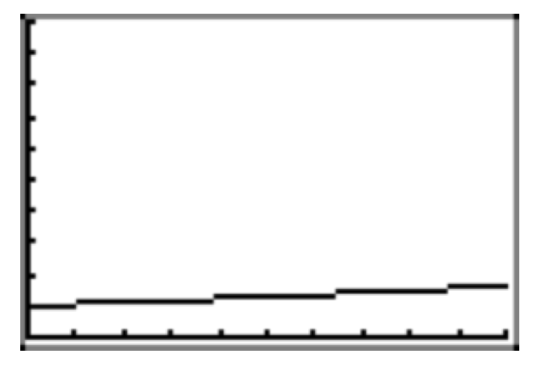
(b) The graph on the interval [0, 100] increases slowly at first, but then increases very rapidly on the second half of the interval.