
2.1: Graphing and slope


- Last updated
- Nov 14, 2021
- Save as PDF

( \newcommand{\kernel}{\mathrm{null}\,}\)
Often, to get an idea of the behavior of an equation, we will make a picture that represents the solutions to the equations called a graph. Let’s have an introduction to graphing so that later we can construct graphs.
A graph represents a visualization of the solutions to an equation.

- The coordinate plane is divided into four quadrants by a horizontal real number line, called the x-axis, and a vertical real number line, called the y-axis.
- The two axes meet at the origin, where x=0 and y=0.
- The x-coordinate is the horizontal distance from the origin and the y-coordinate is the vertical distance from the origin.
- An ordered-pair is where a point in the coordinate plane is located and denoted by (x,y).
- The quadrants are labeled in counter-clockwise starting at the top right.
Locations on the globe are similar to ordered-pairs. Each number is a distance from a central point, the origin, located where the prime meridian and the equator meet. This “origin” is just off the western coast of Africa.
Points and Lines
Plot each ordered-pair and identify the quadrant in which lies the ordered pair: A(−1,−5),B(3,−1),C(−2,3),D(4,2),E(0,4),F(3,0)
Solution
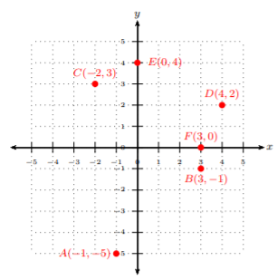
- For point A(−1,−5), notice the x-coordinate is −1. Since the x-coordinate is the horizontal distance from the origin, then we move 1 unit to the left. Looking at the y-coordinate, −5, we see this will be the vertical distance. Hence, we will move 5 units downward from the origin. Starting at the origin, move one unit left, then 5 units down. Point A is in quadrant III.
- For point B(3,−1), notice the x-coordinate is 3. Since the x-coordinate is the horizontal distance from the origin, then we move 3 units to the right. Looking at the y-coordinate, −1, we see this will be the vertical distance. Hence, we will move one unit downward from the origin. Starting at the origin, move 3 units right, then 1 unit down. Point B is in quadrant IV.
- For point C(−2,3), notice the x-coordinate is −2. Since the x-coordinate is the horizontal distance from the origin, then we move 2 units to the left. Looking at the y-coordinate, 3, we see this will be the vertical distance. Hence, we will move 3 units upward from the origin. Starting at the origin, move 2 units left, then 3 units up. Point C is in quadrant III.
- For point D(4,2), notice the x-coordinate is 4. Since the x-coordinate is the horizontal distance from the origin, then we move 4 units to the right. Looking at the y-coordinate, 2, we see this will be the vertical distance. Hence, we will move 2 units upward from the origin. Starting at the origin, move 4 units right, then 2 units up. Point D is in quadrant I.
- For point E(0,4), notice the x-coordinate is 0. Since the x-coordinate is the horizontal distance from the origin, then we move no units horizontally from the origin. Looking at the y-coordinate, 4, we see this will be the vertical distance. Hence, we will move 4 units upward from the origin. Starting at the origin, move 4 units up. Point E is not in any quadrant as it lies on the y-axis.
- For point F(3,0), notice the x-coordinate is 3. Since the x-coordinate is the horizontal distance from the origin, then we move 3 units to the right. Looking at the y-coordinate, 0, we see this will be the vertical distance. Hence, we will move no units vertically from the origin. Starting at the origin, move 3 units right. Point F is not in any quadrant as it lies on the x-axis.
Notice, in points A,B,C, the negative coordinates didn’t imply negative distance from the origin. The negative on these coordinates implies the direction in which we move: horizontal- we move left or right, vertical- we move up or down. If the x-coordinate is negative, then we move to the left. If the y-coordinate is negative, then we move downward.
From Example 2.1.1, with points E and F, we could see that these points did not lie in a quadrant, but on an axis. These are special points on graphs and are called intercepts.
- The x-intercept of a graph is the point(s) where the graph crosses the x-axis, i.e., y=0.
- The y-intercept of a graph is the point(s) where the graph crosses the y-axis, i.e., x=0.
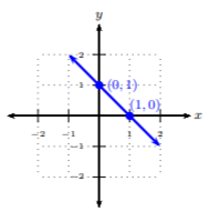
Graph y=1−x by plotting the intercepts.
Solution
To find the x and y-intercepts, we can follow the definition above and find where y=0 and x=0, respectively. Let’s make a table.
Table 2.1.1
| x | y=1−x | (x,y) |
|---|---|---|
| 0=1−x⟹x=1 | 0 | (1,0) |
| 0 | y=1−0=1 | (0,1) |
We can see when y=0,x=1 since 0=1−x only when x=1. Let’s plot the two intercepts from the table. To connect the points, be sure to connect them from smallest x-value to largest x-value, i.e., left to right. Draw the line to fill the grid and put arrows at the ends. It is recommended to purchase a small 6-inch ruler to make nice straight lines.
The main purpose of graphs is not to plot random points, but rather to give a picture of the solutions to an equation. We may have an equation such as y=2x−3 and be interested in the type of solutions that are possible for this equation. We can visualize the solution by making a graph of possible x and y combinations that makes this equation a true statement. We have to start by finding possible x and y combinations. We do this by using a table of values.
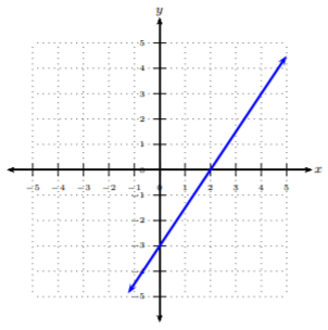
Graph y=2x−3 by plotting points, i.e., by making a T-table.
Solution
Usually, we pick three x-coordinates, and find corresponding y-values. Each x-value being positive, negative, and zero. This is common practice, but not required.
Table 2.1.2
| x | y=2x−3 | (x,y) |
|---|---|---|
| −1 | y=2(−1)−3=−2−3=−5 | (−1,−5) |
| 0 | y=2(0)−3=0−3=−3 | (0,−3) |
| 1 | y=2(1)−3=2−3=−1 | (1,−1) |
Plot the three ordered-pairs from the table. To connect the points, be sure to connect them from smallest x-value to largest x-value, i.e., left to right. Draw the line to fill the grid and put arrows at the ends. It is recommended to purchase a small 6-inch ruler to make nice straight lines.

Graph 2x−3y=6 by plotting points, i.e., by making a T-table.
Solution
Let’s begin by choosing x-values for the table. Notice this equation isn’t as simple as the prior example, so we will have to do a bit of algebra to solve for the y-value. Then fill in the table.
Table 2.1.3
| x | y | (x,y) |
|---|---|---|
| −3 | ||
| 0 | ||
| 3 |
Let’s evaluate 2x−3y=6 for each of the chosen x-values:
x=−3: 2(−3)−3y=6−6−3y+6=6+6−13⋅−3y=12⋅−13y=−4
x=0: 2(0)−3y=60−3y=6−13⋅−3y=6⋅−13y=−2
x=3: 2(3)−3y=66−3y+(−6)=6+(−6)−13⋅−3y=0⋅−13y=0
Now, we fill in the table with y-values and ordered-pairs, and then graph 2x−3y=6.
Table 2.1.4
| x | y | (x,y) |
|---|---|---|
| −3 | −4 | (−3,−4) |
| 0 | −2 | (0,−2) |
| 3 | 0 | (3,0) |

Obtaining the Slope of a Line from its Graph
As we graph lines, we want to identify different properties of lines. One of the most important properties of a line is its slope.
The slope of a line is the measure of the line’s steepness.
- We denote slope with m. One theory from mathematicians that began working with slope was that it was called the modular slope.
- As |m| increases, the line becomes steeper. As |m| decreases, the line becomes flatter.
- A line that rises left to right has a positive slope and and a line that falls left to right has negative slope.
- m is the change of y divided by the change in x, i.e., m=ΔyΔx=Change in yChange in x=riserun
Find the slope from the graph given of the line.
Solution
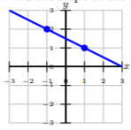
We start at a well-defined point, preferably a point on the y-axis, i.e., the y-intercept. Then count the number of units we rise (up/down) and run (left/right) to reach the next well-defined point. We will start at (0,−3) and reach the next point, (2,0). Notice we rise upward 3 units and run to the right 2 units. Using the ratio, m=riserun, we get the rise to be 3 and the run to be 2: m=riserun=32
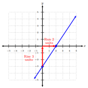
Thus, the slope is 32.
Find the slope from the graph given of the line.

Solution
We start at a well-defined point, preferably a point on the y-axis, i.e., the y-intercept. Then count the number of units we rise (up/down) and run (left/right) to reach the next well-defined point. We will start at (0,2) and reach the next point, (4,1). Notice we rise downward 1 units and run to the right 4 units. Using the ratio, m=riserun, we get the rise to be −1 and the run to be 4: m=riserun=−14
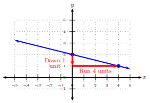
Thus, the slope is −14.
Looking at Examples 2.1.5 and 2.1.6, notice the steepness. Since, in Example 2.1.5, the slope was 32, which is larger than the slope in 2.1.6, Example 2.1.5 is a steeper line than Example 2.1.6. Also, the negative in Example 2.1.6 represents the line falling left to right; hence the negative slope.
When French mathematicians Rene Descartes and Pierre de Fermat first developed the coordinate plane and the idea of graphing lines (and other functions), the y-axis was not a vertical line.
Let’s look at two special cases with lines and their slope.
Find the slope from the graph given of the line.

Solution
In this graph, there is no rise, but the run is 3 units. The slope is 03=0. When the slope of a line is zero, then we know the line is a horizontal line and vise versa.
Find the slope from the graph given of the line.

Solution
In this graph, there is no run, but the rise is 2 units. The slope is 20= undefined. When the slope of a line is undefined, then we know the line is a vertical line and vise versa.
As you can see there is a big difference between having a zero slope and having undefined slope. Remember, slope is a measure of steepness. The first slope is not steep at all. In fact, it is flat. Therefore, it has a zero slope. The second slope can’t get any steeper. It is so steep that there is no number large enough to express the steepness. Hence, being an undefined slope.
Obtaining the Slope of a Line from Two Points
We can find the slope of a line through two points without seeing the points on a graph. We can do this using a slope formula. If the rise is the change in y-values, we can calculate this by subtracting the y-values of a point. Similarly, if run is a change in the x-values, we can calculate this by subtracting the x-values of a point.
Slope, m, is the change of y divided by the change in x, i.e., m=ΔyΔx=Change in yChange in x=riserun=y2−y1x2−x1=y1−y2x1−x2
Find the slope between the two points (−4,3) and (2,−9).
Solution
m=y2−y1x2−x1Substitute in the ordered-pairsm=−9−32−(−4)Simplifym=−126Reducem=−2Slope
Since this slope is −2, then the graph of this line would be falling left to right.
Find the slope between the two points (4,6) and (2,−1).
Solution
m=y2−y1x2−x1Substitute in the ordered-pairsm=−1−62−4Simplifym=−7−2Reduce, dividing by −1m=72Slope
Since this slope is 72, then the graph of this line would be rising left to right.
Find the slope between the two points (−4,−1) and (−4,−5).
Solution
m=y2−y1x2−x1Substitute in the ordered-pairsm=−5−(−1)−4−(−4)Simplifym=−40Undefinedm= undefinedSlope
Since the slope is undefined, then the graph of this line is a vertical line.
Find the slope between the two points (3,1) and (−2,1).
Solution
m=y2−y1x2−x1Substitute in the ordered-pairsm=1−1−2−3Simplifym=0−5Reducem=0Slope
Since the slope is zero, then the graph of this line is a horizontal line.
Find the value of y between the points (2,y) and (5,−1) with slope −3.
Solution
m=y2−y1x2−x1We will plug values into slope formula−3=−1−y5−2Simplify−3=−1−y3Multiply both sides by 33⋅−3=−1−y3⋅3Simplify−9=−1−yIsolate the variable term−9+1=−1−y+1Simplify−8=−yMultiply each side by −1−1⋅−8=−y⋅−18=yValue of y
Find the value of x such that the slope between the points (−3,2) and (x,6) is 25.
Solution
m=y2−y1x2−x1We will plug values into slope formula25=6−2x−(−3)Simplify25=4x+3Multiply both sides by x+3(x+3)⋅25=4x+3⋅(x+3)Simplify25(x+3)=4Distribute25x+65=4Multiply by the LCD =55⋅25x+5⋅65=4⋅5Simplify2x+6=20Isolate the variable term2x+6+(−6)=20+(−6)Simplify2x=14Multiply each side by the reciprocal of 212⋅2x=14⋅12Simplifyx=7Value of x
Graphing and Slope Homework
Find the slope of the line.

Find the slope of the line.
Find the slope of the line.

Find the slope of the line.

Find the slope of the line.
Find the slope of the line.

Find the slope of the line through each ordered-pair.
(−2,10),(−2,−15)
(−15,10),(16,−7)
(10,18),(−11,−10)
(−16,−14),(11,−14)
(−4,14),(−16,8)
(12,−19),(6,14)
(−5,−10),(−5,20)
(−17,19),(10,−7)
(7,−14),(−8,−9)
(−5,7),(−18,14)
(1,2),(−6,−14)
(13,−2),(7,7)
(−3,6),(−20,13)
(13,15),(2,10)
(9,−6),(−7,−7)
(−16,2),(15,−10)
(8,11),(−3,−13)
(11,−2),(1,17)
(−18,−5),(14,−3)
(19,15),(5,11)
Find the value of x or y so that the line through the points has the given slope.
(2,6) and (x,2); m=47
(−3,−2) and (x,6); m=−85
(−8,y) and (−1,1); m=67
(x,−7) and (−9,−9); m=25
(x,5) and (8,0); m=−56
(8,y) and (−2,4); m=−15
(−2,y) and (2,4); m=14
(x,−1) and (−4,6); m=−710
(2,−5) and (3,y); m=6
(6,2) and (x,6); m=−45