
11.4: Graph quadratic functions
- Page ID
- 45113

\( \newcommand{\vecs}[1]{\overset { \scriptstyle \rightharpoonup} {\mathbf{#1}} } \)
\( \newcommand{\vecd}[1]{\overset{-\!-\!\rightharpoonup}{\vphantom{a}\smash {#1}}} \)
\( \newcommand{\id}{\mathrm{id}}\) \( \newcommand{\Span}{\mathrm{span}}\)
( \newcommand{\kernel}{\mathrm{null}\,}\) \( \newcommand{\range}{\mathrm{range}\,}\)
\( \newcommand{\RealPart}{\mathrm{Re}}\) \( \newcommand{\ImaginaryPart}{\mathrm{Im}}\)
\( \newcommand{\Argument}{\mathrm{Arg}}\) \( \newcommand{\norm}[1]{\| #1 \|}\)
\( \newcommand{\inner}[2]{\langle #1, #2 \rangle}\)
\( \newcommand{\Span}{\mathrm{span}}\)
\( \newcommand{\id}{\mathrm{id}}\)
\( \newcommand{\Span}{\mathrm{span}}\)
\( \newcommand{\kernel}{\mathrm{null}\,}\)
\( \newcommand{\range}{\mathrm{range}\,}\)
\( \newcommand{\RealPart}{\mathrm{Re}}\)
\( \newcommand{\ImaginaryPart}{\mathrm{Im}}\)
\( \newcommand{\Argument}{\mathrm{Arg}}\)
\( \newcommand{\norm}[1]{\| #1 \|}\)
\( \newcommand{\inner}[2]{\langle #1, #2 \rangle}\)
\( \newcommand{\Span}{\mathrm{span}}\) \( \newcommand{\AA}{\unicode[.8,0]{x212B}}\)
\( \newcommand{\vectorA}[1]{\vec{#1}} % arrow\)
\( \newcommand{\vectorAt}[1]{\vec{\text{#1}}} % arrow\)
\( \newcommand{\vectorB}[1]{\overset { \scriptstyle \rightharpoonup} {\mathbf{#1}} } \)
\( \newcommand{\vectorC}[1]{\textbf{#1}} \)
\( \newcommand{\vectorD}[1]{\overrightarrow{#1}} \)
\( \newcommand{\vectorDt}[1]{\overrightarrow{\text{#1}}} \)
\( \newcommand{\vectE}[1]{\overset{-\!-\!\rightharpoonup}{\vphantom{a}\smash{\mathbf {#1}}}} \)
\( \newcommand{\vecs}[1]{\overset { \scriptstyle \rightharpoonup} {\mathbf{#1}} } \)
\( \newcommand{\vecd}[1]{\overset{-\!-\!\rightharpoonup}{\vphantom{a}\smash {#1}}} \)
\(\newcommand{\avec}{\mathbf a}\) \(\newcommand{\bvec}{\mathbf b}\) \(\newcommand{\cvec}{\mathbf c}\) \(\newcommand{\dvec}{\mathbf d}\) \(\newcommand{\dtil}{\widetilde{\mathbf d}}\) \(\newcommand{\evec}{\mathbf e}\) \(\newcommand{\fvec}{\mathbf f}\) \(\newcommand{\nvec}{\mathbf n}\) \(\newcommand{\pvec}{\mathbf p}\) \(\newcommand{\qvec}{\mathbf q}\) \(\newcommand{\svec}{\mathbf s}\) \(\newcommand{\tvec}{\mathbf t}\) \(\newcommand{\uvec}{\mathbf u}\) \(\newcommand{\vvec}{\mathbf v}\) \(\newcommand{\wvec}{\mathbf w}\) \(\newcommand{\xvec}{\mathbf x}\) \(\newcommand{\yvec}{\mathbf y}\) \(\newcommand{\zvec}{\mathbf z}\) \(\newcommand{\rvec}{\mathbf r}\) \(\newcommand{\mvec}{\mathbf m}\) \(\newcommand{\zerovec}{\mathbf 0}\) \(\newcommand{\onevec}{\mathbf 1}\) \(\newcommand{\real}{\mathbb R}\) \(\newcommand{\twovec}[2]{\left[\begin{array}{r}#1 \\ #2 \end{array}\right]}\) \(\newcommand{\ctwovec}[2]{\left[\begin{array}{c}#1 \\ #2 \end{array}\right]}\) \(\newcommand{\threevec}[3]{\left[\begin{array}{r}#1 \\ #2 \\ #3 \end{array}\right]}\) \(\newcommand{\cthreevec}[3]{\left[\begin{array}{c}#1 \\ #2 \\ #3 \end{array}\right]}\) \(\newcommand{\fourvec}[4]{\left[\begin{array}{r}#1 \\ #2 \\ #3 \\ #4 \end{array}\right]}\) \(\newcommand{\cfourvec}[4]{\left[\begin{array}{c}#1 \\ #2 \\ #3 \\ #4 \end{array}\right]}\) \(\newcommand{\fivevec}[5]{\left[\begin{array}{r}#1 \\ #2 \\ #3 \\ #4 \\ #5 \\ \end{array}\right]}\) \(\newcommand{\cfivevec}[5]{\left[\begin{array}{c}#1 \\ #2 \\ #3 \\ #4 \\ #5 \\ \end{array}\right]}\) \(\newcommand{\mattwo}[4]{\left[\begin{array}{rr}#1 \amp #2 \\ #3 \amp #4 \\ \end{array}\right]}\) \(\newcommand{\laspan}[1]{\text{Span}\{#1\}}\) \(\newcommand{\bcal}{\cal B}\) \(\newcommand{\ccal}{\cal C}\) \(\newcommand{\scal}{\cal S}\) \(\newcommand{\wcal}{\cal W}\) \(\newcommand{\ecal}{\cal E}\) \(\newcommand{\coords}[2]{\left\{#1\right\}_{#2}}\) \(\newcommand{\gray}[1]{\color{gray}{#1}}\) \(\newcommand{\lgray}[1]{\color{lightgray}{#1}}\) \(\newcommand{\rank}{\operatorname{rank}}\) \(\newcommand{\row}{\text{Row}}\) \(\newcommand{\col}{\text{Col}}\) \(\renewcommand{\row}{\text{Row}}\) \(\newcommand{\nul}{\text{Nul}}\) \(\newcommand{\var}{\text{Var}}\) \(\newcommand{\corr}{\text{corr}}\) \(\newcommand{\len}[1]{\left|#1\right|}\) \(\newcommand{\bbar}{\overline{\bvec}}\) \(\newcommand{\bhat}{\widehat{\bvec}}\) \(\newcommand{\bperp}{\bvec^\perp}\) \(\newcommand{\xhat}{\widehat{\xvec}}\) \(\newcommand{\vhat}{\widehat{\vvec}}\) \(\newcommand{\uhat}{\widehat{\uvec}}\) \(\newcommand{\what}{\widehat{\wvec}}\) \(\newcommand{\Sighat}{\widehat{\Sigma}}\) \(\newcommand{\lt}{<}\) \(\newcommand{\gt}{>}\) \(\newcommand{\amp}{&}\) \(\definecolor{fillinmathshade}{gray}{0.9}\)Let’s recall the parabola from the Functions chapter.
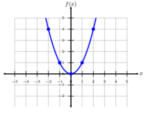
Graph \(f(x)=x^2\).
Solution
Let’s pick five \(x\)-coordinates, and find corresponding \(y\)-values. Each \(x\)-value being positive, negative, and zero. This is common practice, but not required.
| \(x\) | \(f(x)=x^2\) | \((x,f(x))\) |
|---|---|---|
| \(-2\) | \(f(\color{blue}{-2}\color{black}{)}=4\) | \((-2,4)\) |
| \(-1\) | \(f(\color{blue}{-1}\color{black}{)}=1\) | \((-1,1)\) |
| \(0\) | \(f(\color{blue}{0}\color{black}{)}=0\) | \((0,0)\) |
| \(1\) | \(f(\color{blue}{1}\color{black}{)}=1\) | \((1,1)\) |
| \(2\) | \(f(\color{blue}{2}\color{black}{)}=4\) | \((2,4)\) |
Plot the five ordered-pairs from the table. To connect the points, be sure to connect them from smallest \(x\)-value to largest \(x\)-value, i.e., left to right. This graph is called a parabola and since this function is quite common for the \(x^2\)-form, we call it a quadratic (square) function.
Since quadratic functions have a leading term that contains \(x^2\), then a quadratic function’s graph is called a parabola just like in the Functions chapter.
A quadratic function is a polynomial function of the form
\[f(x)=ax^2+bx+c\nonumber\]
where \(a\neq 0\).
In Example 11.4.1 , we plotted points and connected the dots. This is one way of graphing quadratic functions, but not the most efficient. Hence, we can easily graph quadratic functions by finding key elements of the function: vertex, \(x\)-intercepts, and the \(y\)-intercept.
Vertex of a Quadratic Function
The vertex of a quadratic function \(f(x)=ax^2+bx+x\) is given by
\[\left(-\dfrac{b}{2a},f\left(-\dfrac{b}{2a}\right)\right)\nonumber\]
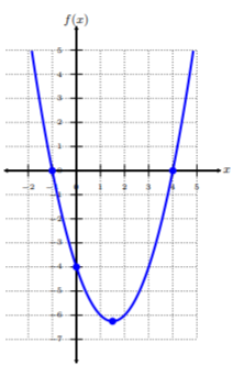
Find the vertex of \(f(x) = x^2 − 3x − 4\).
Solution
The \(x\)-coordinate of the vertex is \(−\dfrac{b}{2a}\) given by the definition. In this case, \(a = 1\), \(b = −3\), and \(c = −4\). Hence,
\[x=-\dfrac{b}{2a}=-\dfrac{-3}{2(1)}=\dfrac{3}{2}\nonumber\]
The \(y\)-coordinate of the vertex is
\[f\left(\dfrac{3}{2}\right)=\left(\dfrac{3}{2}\right)^2-3\left(\dfrac{3}{2}\right)-4=-\dfrac{25}{4}\nonumber\]
Thus, the vertex of \(f(x)\) is at \(\left(\dfrac{3}{2},-\dfrac{25}{4}\right)\). Let’s take a look at the graph and verify this is the location of the vertex. We see the vertex is, in fact, located at \(\left(\dfrac{3}{2},-\dfrac{25}{4}\right)\). Additionally, we see the parabola intersects the \(x\)-axis at \(x = −1\) and \(x = 4\), and the \(y\)-axis at \((0, −4)\).
Graph Quadratic Functions by its Properties
To graph a quadratic function, \(f(x) = ax^2 + bx + x\), by its properties, we obtain key properties.
Property 1. The direction of the parabola.
- If \(a > 0\), then the graph is an upward parabola.
- If \(a < 0\), then the graph is a downward parabola.
Property 2. The vertex: \(\left(-\dfrac{b}{2a},f\left(-\dfrac{b}{2a}\right)\right)\)
Property 3. The \(y\)-intercept: \((0, f(0))\)
Property 4. The \(x\)-intercepts: \((x, 0)\), i.e., where \(f(x) = 0\), also known as the zeros of \(f(x)\).
Property 5. The axis of symmetry: \(x = −\dfrac{b}{2a}\)
The axis of symmetry is a vertical line that intersects the vertex of the parabola. Hence, the line \(x=-\dfrac{b}{2a}\). The axis of symmetry essentially “cuts” the parabola in half and the parabola is symmetrical about this axis.
Using the properties, graph \(f(x)=x^2+4x+3\).
Solution
Property 1. The direction of the parabola. Since \(a = 1\) and \(a > 0\), then \(f(x)\) is an upwards parabola.
Property 2. Find the vertex. We use the formula to find the vertex, where \(a = 1\) and \(b = 4\). \[\begin{array}{rl}x=-\dfrac{b}{2a}&\text{Plug-n-chug} \\ x=-\dfrac{\color{blue}{4}}{\color{blue}{(2)(1)}}&\color{black}{\text{Simplify}} \\ x=-2&\text{The }x\text{-coordinate of the vertex}\end{array}\nonumber\] Next, we find the \(y\)-coordinate of the vertex by obtaining \(f(-2)\). \[\begin{array}{rl}f(x)=x^2+4x+3&\text{Plug-n-chug} \\ f(\color{blue}{-2}\color{black}{)}=(\color{blue}{-2}\color{black}{)}^2+4(\color{blue}{-2}\color{black}{)}+3&\text{Evaluate} \\ f(-2)=-1&\text{The }y\text{-coordinate of the vertex}\end{array}\nonumber\] Hence, the vertex is \((-2,-1)\).
Property 3. Find the \(y\)-intercept. We can find the \(y\)-intercept by obtaining \(f(0)\). \[\begin{array}{rl}f(x)=x^2+4x+3&\text{Plug-n-chug }x=0 \\ f(\color{blue}{0}\color{black}{)}=\color{blue}{0}\color{black}{^2}+4(\color{blue}{0}\color{black}{)}+3 &\text{Evaluate} \\ f(0)=3&\text{The }y\text{-intercept}\end{array}\nonumber\] Hence, the \(y\)-intercept is \((0,3)\).
Property 4. Find the \(x\)-intercepts. We can find the \(x\)-intercept by obtaining where \(f(x) = 0\). \[\begin{array}{rl} f(x)=x^2+4x+3&\text{Plug-n-chug }f(x)=0 \\ 0=x^2+4x+3&\text{Factor} \\ 0=(x+3)(x+1)&\text{Apply the zero product rule} \\ x+3=0\quad\text{and}\quad x+1=0&\text{Solve each equation} \\ x=-3\quad\text{and}\quad x=-1&\text{The }x\text{-intercepts}\end{array}\nonumber\] Hence, the \(x\)-intercepts are \((-3,0)\) and \((-1,0)\).
Property 5. Find the axis of symmetry. We see from the vertex in Property 2. \(x = −2\). Thus, the axis of symmetry is the vertical line \(x = −2\).
Let’s graph all the properties and label each property.
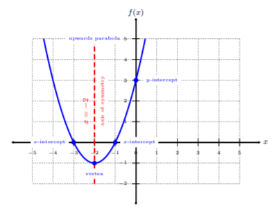
So, we verify that \(f(x)\) is an upwards parabola with \(x\)-intercepts \((−3, 0)\) and \((−1, 0)\), \(y\)-intercept \((0, 3)\), vertex \((−2, −1)\), and axis of symmetry \(x = −2\).
Using the properties, graph \(g(x) = −3x^2 + 12x − 9\).
Solution
Property 1. The direction of the parabola. Since \(a = −3\) and \(a < 0\), then \(g(x)\) is an downwards parabola.
Property 2. Find the vertex. We use the formula to find the vertex, where \(a = −3\) and \(b = 12\). \[\begin{array}{rl}x=-\dfrac{b}{2a}&\text{Plug-n-chug} \\ x=-\dfrac{\color{blue}{12}}{\color{blue}{2(-3)}}&\text{Simplify} \\ x=2&\text{The }x\text{-coordinate of the vertex}\end{array}\nonumber\] Next, we find the \(y\)-coordinate of the vertex by obtaining \(g(2)\). \[\begin{array}{rl}g(x)=-3x^2+12x-9&\text{Plug-n-chug} \\ g(\color{blue}{2}\color{black}{)}=-3(\color{blue}{2}\color{black}{)}^2+12(\color{blue}{2}\color{black}{)}-9&\text{Evaluate} \\ g(2)=3&\text{The }y\text{-coordinate of the vertex}\end{array}\nonumber\] Hence, the vertex is \((2,3)\).
Property 3. Find the \(y\)-intercept. We can find the \(y\)-intercept by obtaining \(f(0)\). \[\begin{array}{rl}g(x)=-3x^2+12x-9&\text{ Plug-n-chug }x=0 \\ g(\color{blue}{0}\color{black}{)}=-3\color{blue}{0}\color{black}{^2}+12(\color{blue}{0}\color{black}{)}-9&\text{Evaluate} \\ g(0)=-9&\text{The }y\text{-intercept}\end{array}\nonumber\] Hence, the \(y\)-intercept is \((0,-9)\).
Property 4. Find the \(x\)-intercepts. We can find the \(x\)-intercept by obtaining where \(g(x) = 0\). \[\begin{array}{rl} g(x)=-3x^2+12x-9&\text{Plug-n-chug }g(x)=0 \\ 0=-3x^2+12x-9&\text{Factor a GCF of }-3 \\ =-3(x^2-4x+3)&\text{Divide each side by }-3\text{, then factor} \\ 0=(x-3)(x-1)&\text{Apply the zero product rule} \\ x-3=0\quad\text{and}\quad x-1=0&\text{Solve each equation} \\ x=3\quad\text{and}\quad x=1&\text{The }x\text{-intercepts}\end{array}\nonumber\] Hence, the \(x\)-intercepts are \((3,0)\) and \((1,0)\).
Property 5. Find the axis of symmetry. We see from the vertex in Property 2. \(x = 2\). Thus, the axis of symmetry is the vertical line \(x = 2\).
Let’s graph all the properties and label each property.
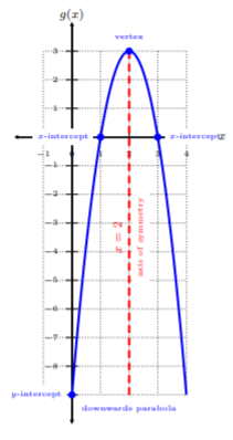
So, we verify that \(g(x)\) is an downwards parabola with \(x\)-intercepts \((3, 0)\) and \((1, 0)\), \(y\)-intercept \((0, −9)\), vertex \((2, 3)\), and axis of symmetry \(x = 2\).
Graph Quadratic Functions by Transformations
A quadratic function in vertex form is given as
\[f(x)=a(x-h)^2+k,\nonumber\]
where the domain consists of all real numbers and \((h, k)\) is the vertex.
Recall. In the chapter with rational functions, we graphed rational functions with horizontal and vertical shift. Let’s take this one step further, and graph quadratic functions with not only horizontal and vertical shifts, but also with a stretch or compression.
Given \(f(x)\) is the quadratic function in vertex form
\[f(x)=a(x-h)^2+k,\nonumber\]
horizontal and vertical shifts, and vertical stretches or compressions of \(f(x)\) are described below:
| \(f(x-h)\) | \(f(x)\pm k\) | \(af(x)\) | |
|---|---|---|---|
| Transformation | Horizontal shift | Vertical shift | Vertical stretch or compression |
| Units | \(h>0\): Shift \(h\) units to the right \(h<0\): Shift \(h\) units to the left |
\(k>0\): Shift \(k\) units upwards \(k<0\): Shift \(k\) units downwards |
\(|a|>1\): Multiply all outputs by \(a\); vertical stretch \(0<|a|<1\): Multiply all outputs by \(a\); vertical compression |
Recall from the previous subsection, if \(a > 0\), the parabola is upward and if \(a < 0\), the parabola is downward.
Using the library function \(f(x)=x^2\), graph \(g(x)=x^2+2\).
Solution
We start by noticing we are adding \(2\) to \(f(x)\), i.e., \(g(x) = f(x) + 2\):
\[\begin{aligned}g(x)&=x^2+2 \\ g(x)&=f(x)+2\end{aligned}\]
This means, from the table, \(g(x)\) has a vertical shift by \(2\) units upward. Let’s start with \(f(x) = x^2\), and then shift \(f(x)\) \(2\) units upward to obtain \(g(x)\):
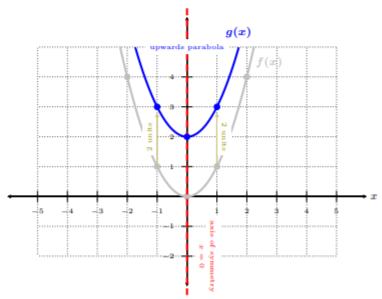
We can see that the blue solid graph is \(g(x)\), where \(g(x)\) is an upward parabola, the axis of symmetry is \(x = 0\). Notice, all points on \(f(x)\) shifted upwards by \(2\) units. We can use the well-defined points of the library function \(f(x) = x^2\) to transform into \(g(x)\).
Using the library function \(f(x) = x^2\), graph \(h(x) = (x − 3)^2 + 2\).
Solution
We start by noticing we are adding \(2\) to \(f(x)\) and subtracting \(3\) from the input \(x\), i.e., \(h(x) = f(x − 3) + 2\):
\[\begin{aligned}h(x)&=(x-3)^2+2 \\ h(x)&=f(x-3)+2\end{aligned}\]
This means, from the table, \(h(x)\) has a horizontal shift to the right by \(3\) units, and vertical shift by \(2\) units upward. Let’s start with \(f(x) = x^2\), and then shift \(f(x)\) \(3\) units to the right, and \(2\) units upward to obtain \(h(x)\):
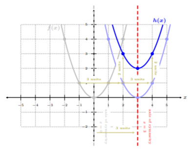
We can see that the blue solid graph is \(h(x)\), where \(h(x)\) is an upward parabola, the axis of symmetry is \(x = 3\). Notice, all points on \(f(x)\) shifted right by \(3\) units and upwards by \(2\) units. We can use the well-defined points of the library function \(f(x) = x^2\) to transform into \(h(x)\).
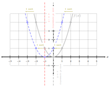
Using the library function \(f(x) = x^2\), graph \(k(x) = −2(x + 1)^2 − 3\).
Solution
We start by noticing we are subtracting \(3\) from \(f(x)\), vertically stretching by a factor of \(−2\), and adding \(1\) to the input \(x\), i.e., \(k(x) = −2\cdot f(x + 1) − 3\):
\[\begin{aligned} k(x)&=-2(x+1)^2-3 \\ k(x)&=-2\cdot f(x+1)-3\end{aligned}\]
This means, from the table, \(k(x)\) has a horizontal shift to the left by \(1\) unit, a vertical stretch by a factor of \(−2\), and a vertical shift by \(3\) units downward. Let’s start with \(f(x) = x^2\), and then apply these transformations to obtain \(k(x)\). Since there are three transformations, it is best we split this up into three steps.
Step 1. Graph the library function, \(f(x)=x^2\), and apply the horizontal shift: \(f(x+1)\).
Step 2. Graph \(f(x + 1)\) from Step 1., and apply the vertical stretch, i.e., multiply the \(y\)-coordinates of the well-defined ordered pairs by \(−2\): \(−2\cdot f(x + 1)\)
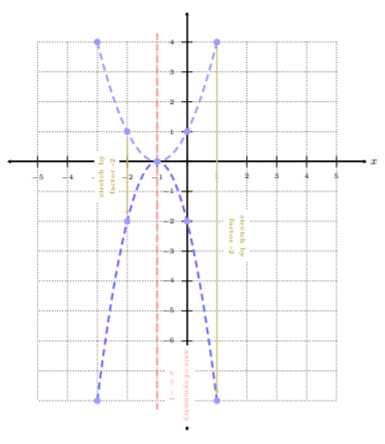
Step 3. Graph \(−2\cdot f(x + 1)\) from Step 2., and apply the vertical shift: \(−2\cdot f(x + 1) − 3\)
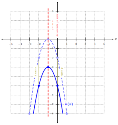
We can see that the blue solid graph is \(k(x)\), where \(k(x)\) is an downward parabola, the axis of symmetry is \(x = −1\). Notice, all points on \(f(x)\) shifted left by \(1\) unit, stretched by a factor of \(−2\), and shifted downwards by \(3\) units.
Notice with three transformations, it can get tedious and tricky. The best route to apply multiple transformations is to follow order of operations, e.g., first parenthesis, multiplication/division, and then addition/subtraction. With transformations, this translates to
Step 1. Apply the horizontal shift
Step 2. Vertically stretch or compress the function
Step 3. Lastly, apply the vertical shift
A way to remember the order in which we apply the transformations is \(hak\): first the \(h\), then \(a\), lastly, \(k\).
Graph Quadratic Functions Homework
Graph the quadratic function using the properties. Be sure to label your graph with all properties.
\(f(x)=x^2-2x-8\)
\(f(x)=2x^2-12x+10\)
\(f(x)=-2x^2+12x-18\)
\(f(x)=-3x^2+24x-45\)
\(f(x)=-x^2+4x+5\)
\(f(x)=-x^2+6x-5\)
\(f(x)=-2x^2+16x-24\)
\(f(x)=3x^2+12x+9\)
\(f(x)=5x^2-40x+75\)
\(f(x)=-5x^2-60x-175\)
\(f(x)=x^2-2x-3\)
\(f(x)=2x^2-12x+16\)
\(f(x)=-2x^2+12x-10\)
\(f(x)=-3x^2+12x-9\)
\(f(x)=-x^2+4x-3\)
\(f(x)=-2x^2+16x-30\)
\(f(x)=2x^2+4x-6\)
\(f(x)=5x^2+30x+45\)
\(f(x)=5x^2+20x+15\)
\(f(x)=-5x^2+20x-15\)
Starting with the library function \(y=x^2\), state the function, \(f(x)\), given its transformation(s).
vertically stretched by a factor of \(3\) and shifted right \(1\)
vertically stretched by a factor of \(-2\), and shifted left \(3\)
vertically compressed by a factor of \(\dfrac{1}{3}\)
vertically stretched by a factor of \(2\) and shifted right \(4\)
vertically stretched by a factor of \(4\), shifted left \(4\)
vertically compressed by a factor of \(−\dfrac{1}{2}\) and shifted upward by \(3\) units
vertically stretched by a factor of \(3\) and shifted down \(4\)
vertically stretched by a factor of \(2\), shifted right \(3\), and shifted up \(1\)
Starting with the library function \(y=x^2\), graph the function using transformations.
\(g(x)=-\dfrac{1}{2}(x+7)^2\)
\(g(x)=2(x-1)^2-2\)
\(y=\dfrac{1}{5}(x-2)^2\)
\(f(x)=\dfrac{1}{2}(x+2)^2+9\)
\(f(x)=2(x+4)^2-5\)
\(f(x)=-2(x-4)^2+7\)
\(g(x)=2(x-3)^2-2\)
\(g(x)=-\dfrac{1}{2}(x+5)^2\)
\(f(x)=\dfrac{1}{2}(x+4)^2+8\)
\(f(x)=-2(x-8)^2+7\)