3.5: Rational Functions

Last updated
Save as PDF

Page ID: 239

$ \newcommand{\vecs}[1]{\overset { \scriptstyle \rightharpoonup} {\mathbf{#1}} } $

$ \newcommand{\vecd}[1]{\overset{-\!-\!\rightharpoonup}{\vphantom{a}\smash {#1}}} $

$ \newcommand{\dsum}{\displaystyle\sum\limits} $

$ \newcommand{\dint}{\displaystyle\int\limits} $

$ \newcommand{\dlim}{\displaystyle\lim\limits} $

$ \newcommand{\id}{\mathrm{id}}$ $ \newcommand{\Span}{\mathrm{span}}$

( \newcommand{\kernel}{\mathrm{null}\,}\) $ \newcommand{\range}{\mathrm{range}\,}$

$ \newcommand{\RealPart}{\mathrm{Re}}$ $ \newcommand{\ImaginaryPart}{\mathrm{Im}}$

$ \newcommand{\Argument}{\mathrm{Arg}}$ $ \newcommand{\norm}[1]{\| #1 \|}$

$ \newcommand{\inner}[2]{\langle #1, #2 \rangle}$

$ \newcommand{\Span}{\mathrm{span}}$

$ \newcommand{\id}{\mathrm{id}}$

$ \newcommand{\Span}{\mathrm{span}}$

$ \newcommand{\kernel}{\mathrm{null}\,}$

$ \newcommand{\range}{\mathrm{range}\,}$

$ \newcommand{\RealPart}{\mathrm{Re}}$

$ \newcommand{\ImaginaryPart}{\mathrm{Im}}$

$ \newcommand{\Argument}{\mathrm{Arg}}$

$ \newcommand{\norm}[1]{\| #1 \|}$

$ \newcommand{\inner}[2]{\langle #1, #2 \rangle}$

$ \newcommand{\Span}{\mathrm{span}}$ $ \newcommand{\AA}{\unicode[.8,0]{x212B}}$

$ \newcommand{\vectorA}[1]{\vec{#1}} % arrow$

$ \newcommand{\vectorAt}[1]{\vec{\text{#1}}} % arrow$

$ \newcommand{\vectorB}[1]{\overset { \scriptstyle \rightharpoonup} {\mathbf{#1}} } $

$ \newcommand{\vectorC}[1]{\textbf{#1}} $

$ \newcommand{\vectorD}[1]{\overrightarrow{#1}} $

$ \newcommand{\vectorDt}[1]{\overrightarrow{\text{#1}}} $

$ \newcommand{\vectE}[1]{\overset{-\!-\!\rightharpoonup}{\vphantom{a}\smash{\mathbf {#1}}}} $

$ \newcommand{\vecs}[1]{\overset { \scriptstyle \rightharpoonup} {\mathbf{#1}} } $

$\newcommand{\longvect}{\overrightarrow}$

$ \newcommand{\vecd}[1]{\overset{-\!-\!\rightharpoonup}{\vphantom{a}\smash {#1}}} $

$\newcommand{\ket}[1]{\left| #1 \right>}$
$\newcommand{\bra}[1]{\left< #1 \right|}$
$\newcommand{\braket}[2]{\left< #1 \vphantom{#2} \right| \left. #2 \vphantom{#1} \right>}$
$\newcommand{\braopket}[3]{\left< #1 \vphantom{#2}\vphantom{#3} \right| #2 \vphantom{#1}\vphantom{#3} \left| #3 \vphantom{#1}\vphantom{#2} \right>}$
$\newcommand{\qmvec}[1]{\mathbf{\vec{#1}}}$
$\newcommand{\op}[1]{\hat{\mathbf{#1}}}$
$\newcommand{\expect}[1]{\langle #1 \rangle}$
$\newcommand{\dfn}[1]{\emph{\textbf{#1}}}$

$\newcommand{\avec}{\mathbf a}$ $\newcommand{\bvec}{\mathbf b}$ $\newcommand{\cvec}{\mathbf c}$ $\newcommand{\dvec}{\mathbf d}$ $\newcommand{\dtil}{\widetilde{\mathbf d}}$ $\newcommand{\evec}{\mathbf e}$ $\newcommand{\fvec}{\mathbf f}$ $\newcommand{\nvec}{\mathbf n}$ $\newcommand{\pvec}{\mathbf p}$ $\newcommand{\qvec}{\mathbf q}$ $\newcommand{\svec}{\mathbf s}$ $\newcommand{\tvec}{\mathbf t}$ $\newcommand{\uvec}{\mathbf u}$ $\newcommand{\vvec}{\mathbf v}$ $\newcommand{\wvec}{\mathbf w}$ $\newcommand{\xvec}{\mathbf x}$ $\newcommand{\yvec}{\mathbf y}$ $\newcommand{\zvec}{\mathbf z}$ $\newcommand{\rvec}{\mathbf r}$ $\newcommand{\mvec}{\mathbf m}$ $\newcommand{\zerovec}{\mathbf 0}$ $\newcommand{\onevec}{\mathbf 1}$ $\newcommand{\real}{\mathbb R}$ $\newcommand{\twovec}[2]{\left[\begin{array}{r}#1 \\ #2 \end{array}\right]}$ $\newcommand{\ctwovec}[2]{\left[\begin{array}{c}#1 \\ #2 \end{array}\right]}$ $\newcommand{\threevec}[3]{\left[\begin{array}{r}#1 \\ #2 \\ #3 \end{array}\right]}$ $\newcommand{\cthreevec}[3]{\left[\begin{array}{c}#1 \\ #2 \\ #3 \end{array}\right]}$ $\newcommand{\fourvec}[4]{\left[\begin{array}{r}#1 \\ #2 \\ #3 \\ #4 \end{array}\right]}$ $\newcommand{\cfourvec}[4]{\left[\begin{array}{c}#1 \\ #2 \\ #3 \\ #4 \end{array}\right]}$ $\newcommand{\fivevec}[5]{\left[\begin{array}{r}#1 \\ #2 \\ #3 \\ #4 \\ #5 \\ \end{array}\right]}$ $\newcommand{\cfivevec}[5]{\left[\begin{array}{c}#1 \\ #2 \\ #3 \\ #4 \\ #5 \\ \end{array}\right]}$ $\newcommand{\mattwo}[4]{\left[\begin{array}{rr}#1 \amp #2 \\ #3 \amp #4 \\ \end{array}\right]}$ $\newcommand{\laspan}[1]{\text{Span}\{#1\}}$ $\newcommand{\bcal}{\cal B}$ $\newcommand{\ccal}{\cal C}$ $\newcommand{\scal}{\cal S}$ $\newcommand{\wcal}{\cal W}$ $\newcommand{\ecal}{\cal E}$ $\newcommand{\coords}[2]{\left\{#1\right\}_{#2}}$ $\newcommand{\gray}[1]{\color{gray}{#1}}$ $\newcommand{\lgray}[1]{\color{lightgray}{#1}}$ $\newcommand{\rank}{\operatorname{rank}}$ $\newcommand{\row}{\text{Row}}$ $\newcommand{\col}{\text{Col}}$ $\renewcommand{\row}{\text{Row}}$ $\newcommand{\nul}{\text{Nul}}$ $\newcommand{\var}{\text{Var}}$ $\newcommand{\corr}{\text{corr}}$ $\newcommand{\len}[1]{\left|#1\right|}$ $\newcommand{\bbar}{\overline{\bvec}}$ $\newcommand{\bhat}{\widehat{\bvec}}$ $\newcommand{\bperp}{\bvec^\perp}$ $\newcommand{\xhat}{\widehat{\xvec}}$ $\newcommand{\vhat}{\widehat{\vvec}}$ $\newcommand{\uhat}{\widehat{\uvec}}$ $\newcommand{\what}{\widehat{\wvec}}$ $\newcommand{\Sighat}{\widehat{\Sigma}}$ $\newcommand{\lt}{<}$ $\newcommand{\gt}{>}$ $\newcommand{\amp}{&}$ $\definecolor{fillinmathshade}{gray}{0.9}$

1. Rational Functions (Definition)

is a quotient of polynomials $\dfrac{P(x)}{Q(x)}$.

are all Rational Functions

\[\{x | x \text{ is not }1 \text{ or } -1\}.\]

2. Vertical Asymptotes

of a rational function occurs where the denominator is 0.

\[f(x) \rightarrow\infty.\]

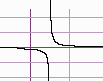
Four Types of Vertical Asymptotes

Below are the four types of vertical asymptotes:

3. Horizontal Asymptotes

and we have the the left and right behavior of the graph is a horizontal line $y = 3$.

4. Oblique Asymptotes

Consider the function

\[f(x) = \dfrac{(x^2 - 3x - 4)}{(x + 3)}\]

$alt$

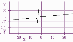
$f(x)$ does not have a horizontal asymptote, since

\[\dfrac{x^2}{x}= x \]

is not a constant, but we see (on the calculator) that the left and right behavior of the curve is like a line. Our goal is to find the equation of this line.

We use synthetic division to see that

\[\dfrac{(x^2 - 3x - 4)}{(x + 3)} = x - 6 + \dfrac{14}{(x+3)}.\]

For very large $x$,

\[\dfrac{14}{x} + 3\]

is very small, hence $f(x)$ is approximately equal to

\[x - 6\]

on the far left and far right of the graph. We call this line an Oblique Asymptote.

To graph, we see that there is a vertical asymptote at

\[x = -3\]

with behavior:

left down and right up

The graph has x-intercepts at 4 and -1, and a y intercept at $-\frac{4}{3}$.

\[\dfrac{(x^3 + 8)}{(x^2 - 3x - 4)}\]

5. Rational Functions With Common Factors

Consider the graph of

\[y = \dfrac{x-1}{x-1}\]

$alt$

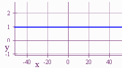
What is wrong with the picture? When

\[f(x) = \dfrac{g(x)(x - r)}{h(x)(x - r)}\]

with neither $g(r)$ nor $h(r)$ zero, the graph will have a hole at $x = r$. We call this hole a removable discontinuity.

at $(2,2)$.

We end our discussion with a list of steps for graphing rational functions.

Steps in graphing rational functions:

Step 1 Plug in $x = 0$ to find the y-intercept
Step 2 Factor the numerator and denominator. Cancel any common factors remember to put in the appropriate holes if necessary.
Step 3 Set the numerator = 0 to find the x-intercepts
Step 4 Set the denominator = 0 to find the vertical asymptotes. Then plug in nearby values to fine the left and right behavior of the vertical asymptotes.
Step 5 If the degree of the numerator = degree of the denominator then the graph has a horizontal asymptote. To determine the value of the horizontal asymptote, divide the term highest power of the numerator by the term of highest power of the denominator.
If the degree of the numerator = degree of the denominator + 1, then use polynomial or synthetic division to determine the equation of the oblique asymptote.
Step 6 Graph it!

Larry Green (Lake Tahoe Community College)

Integrated by Justin Marshall.

Search

Text Color

Text Size

Margin Size

Font Type