
12.2: Nyquist Criterion for Stability
- Page ID
- 6545
\( \newcommand{\vecs}[1]{\overset { \scriptstyle \rightharpoonup} {\mathbf{#1}} } \)
\( \newcommand{\vecd}[1]{\overset{-\!-\!\rightharpoonup}{\vphantom{a}\smash {#1}}} \)
\( \newcommand{\dsum}{\displaystyle\sum\limits} \)
\( \newcommand{\dint}{\displaystyle\int\limits} \)
\( \newcommand{\dlim}{\displaystyle\lim\limits} \)
\( \newcommand{\id}{\mathrm{id}}\) \( \newcommand{\Span}{\mathrm{span}}\)
( \newcommand{\kernel}{\mathrm{null}\,}\) \( \newcommand{\range}{\mathrm{range}\,}\)
\( \newcommand{\RealPart}{\mathrm{Re}}\) \( \newcommand{\ImaginaryPart}{\mathrm{Im}}\)
\( \newcommand{\Argument}{\mathrm{Arg}}\) \( \newcommand{\norm}[1]{\| #1 \|}\)
\( \newcommand{\inner}[2]{\langle #1, #2 \rangle}\)
\( \newcommand{\Span}{\mathrm{span}}\)
\( \newcommand{\id}{\mathrm{id}}\)
\( \newcommand{\Span}{\mathrm{span}}\)
\( \newcommand{\kernel}{\mathrm{null}\,}\)
\( \newcommand{\range}{\mathrm{range}\,}\)
\( \newcommand{\RealPart}{\mathrm{Re}}\)
\( \newcommand{\ImaginaryPart}{\mathrm{Im}}\)
\( \newcommand{\Argument}{\mathrm{Arg}}\)
\( \newcommand{\norm}[1]{\| #1 \|}\)
\( \newcommand{\inner}[2]{\langle #1, #2 \rangle}\)
\( \newcommand{\Span}{\mathrm{span}}\) \( \newcommand{\AA}{\unicode[.8,0]{x212B}}\)
\( \newcommand{\vectorA}[1]{\vec{#1}} % arrow\)
\( \newcommand{\vectorAt}[1]{\vec{\text{#1}}} % arrow\)
\( \newcommand{\vectorB}[1]{\overset { \scriptstyle \rightharpoonup} {\mathbf{#1}} } \)
\( \newcommand{\vectorC}[1]{\textbf{#1}} \)
\( \newcommand{\vectorD}[1]{\overrightarrow{#1}} \)
\( \newcommand{\vectorDt}[1]{\overrightarrow{\text{#1}}} \)
\( \newcommand{\vectE}[1]{\overset{-\!-\!\rightharpoonup}{\vphantom{a}\smash{\mathbf {#1}}}} \)
\( \newcommand{\vecs}[1]{\overset { \scriptstyle \rightharpoonup} {\mathbf{#1}} } \)
\( \newcommand{\vecd}[1]{\overset{-\!-\!\rightharpoonup}{\vphantom{a}\smash {#1}}} \)
\(\newcommand{\avec}{\mathbf a}\) \(\newcommand{\bvec}{\mathbf b}\) \(\newcommand{\cvec}{\mathbf c}\) \(\newcommand{\dvec}{\mathbf d}\) \(\newcommand{\dtil}{\widetilde{\mathbf d}}\) \(\newcommand{\evec}{\mathbf e}\) \(\newcommand{\fvec}{\mathbf f}\) \(\newcommand{\nvec}{\mathbf n}\) \(\newcommand{\pvec}{\mathbf p}\) \(\newcommand{\qvec}{\mathbf q}\) \(\newcommand{\svec}{\mathbf s}\) \(\newcommand{\tvec}{\mathbf t}\) \(\newcommand{\uvec}{\mathbf u}\) \(\newcommand{\vvec}{\mathbf v}\) \(\newcommand{\wvec}{\mathbf w}\) \(\newcommand{\xvec}{\mathbf x}\) \(\newcommand{\yvec}{\mathbf y}\) \(\newcommand{\zvec}{\mathbf z}\) \(\newcommand{\rvec}{\mathbf r}\) \(\newcommand{\mvec}{\mathbf m}\) \(\newcommand{\zerovec}{\mathbf 0}\) \(\newcommand{\onevec}{\mathbf 1}\) \(\newcommand{\real}{\mathbb R}\) \(\newcommand{\twovec}[2]{\left[\begin{array}{r}#1 \\ #2 \end{array}\right]}\) \(\newcommand{\ctwovec}[2]{\left[\begin{array}{c}#1 \\ #2 \end{array}\right]}\) \(\newcommand{\threevec}[3]{\left[\begin{array}{r}#1 \\ #2 \\ #3 \end{array}\right]}\) \(\newcommand{\cthreevec}[3]{\left[\begin{array}{c}#1 \\ #2 \\ #3 \end{array}\right]}\) \(\newcommand{\fourvec}[4]{\left[\begin{array}{r}#1 \\ #2 \\ #3 \\ #4 \end{array}\right]}\) \(\newcommand{\cfourvec}[4]{\left[\begin{array}{c}#1 \\ #2 \\ #3 \\ #4 \end{array}\right]}\) \(\newcommand{\fivevec}[5]{\left[\begin{array}{r}#1 \\ #2 \\ #3 \\ #4 \\ #5 \\ \end{array}\right]}\) \(\newcommand{\cfivevec}[5]{\left[\begin{array}{c}#1 \\ #2 \\ #3 \\ #4 \\ #5 \\ \end{array}\right]}\) \(\newcommand{\mattwo}[4]{\left[\begin{array}{rr}#1 \amp #2 \\ #3 \amp #4 \\ \end{array}\right]}\) \(\newcommand{\laspan}[1]{\text{Span}\{#1\}}\) \(\newcommand{\bcal}{\cal B}\) \(\newcommand{\ccal}{\cal C}\) \(\newcommand{\scal}{\cal S}\) \(\newcommand{\wcal}{\cal W}\) \(\newcommand{\ecal}{\cal E}\) \(\newcommand{\coords}[2]{\left\{#1\right\}_{#2}}\) \(\newcommand{\gray}[1]{\color{gray}{#1}}\) \(\newcommand{\lgray}[1]{\color{lightgray}{#1}}\) \(\newcommand{\rank}{\operatorname{rank}}\) \(\newcommand{\row}{\text{Row}}\) \(\newcommand{\col}{\text{Col}}\) \(\renewcommand{\row}{\text{Row}}\) \(\newcommand{\nul}{\text{Nul}}\) \(\newcommand{\var}{\text{Var}}\) \(\newcommand{\corr}{\text{corr}}\) \(\newcommand{\len}[1]{\left|#1\right|}\) \(\newcommand{\bbar}{\overline{\bvec}}\) \(\newcommand{\bhat}{\widehat{\bvec}}\) \(\newcommand{\bperp}{\bvec^\perp}\) \(\newcommand{\xhat}{\widehat{\xvec}}\) \(\newcommand{\vhat}{\widehat{\vvec}}\) \(\newcommand{\uhat}{\widehat{\uvec}}\) \(\newcommand{\what}{\widehat{\wvec}}\) \(\newcommand{\Sighat}{\widehat{\Sigma}}\) \(\newcommand{\lt}{<}\) \(\newcommand{\gt}{>}\) \(\newcommand{\amp}{&}\) \(\definecolor{fillinmathshade}{gray}{0.9}\)The Nyquist criterion is a graphical technique for telling whether an unstable linear time invariant system can be stabilized using a negative feedback loop. We will look a little more closely at such systems when we study the Laplace transform in the next topic. For this topic we will content ourselves with a statement of the problem with only the tiniest bit of physical context.
You have already encountered linear time invariant systems in 18.03 (or its equivalent) when you solved constant coefficient linear differential equations.
System Functions
A linear time invariant system has a system function which is a function of a complex variable. Typically, the complex variable is denoted by \(s\) and a capital letter is used for the system function.
Let \(G(s)\) be such a system function. We will make a standard assumption that \(G(s)\) is meromorphic with a finite number of (finite) poles. This assumption holds in many interesting cases. For example, quite often \(G(s)\) is a rational function \(Q(s)/P(s)\) (\(Q\) and \(P\) are polynomials).
We will be concerned with the stability of the system.
The system with system function \(G(s)\) is called stable if all the poles of \(G\) are in the left half-plane. That is, if all the poles of \(G\) have negative real part.
The system is called unstable if any poles are in the right half-plane, i.e. have positive real part.
For the edge case where no poles have positive real part, but some are pure imaginary we will call the system marginally stable. This case can be analyzed using our techniques. For our purposes it would require and an indented contour along the imaginary axis. If we have time we will do the analysis.
Is the system with system function \(G(s) = \dfrac{s}{(s + 2) (s^2 + 4s + 5)}\) stable?
Solution
The poles are \(-2, -2\pm i\). Since they are all in the left half-plane, the system is stable.
Is the system with system function \(G(s) = \dfrac{s}{(s^2 - 4) (s^2 + 4s + 5)}\) stable?
Solution
The poles are \(\pm 2, -2 \pm i\). Since one pole is in the right half-plane, the system is unstable.
Is the system with system function \(G(s) = \dfrac{s}{(s + 2) (s^2 + 4)}\) stable?
Solution
The poles are \(-2, \pm 2i\). There are no poles in the right half-plane. Since there are poles on the imaginary axis, the system is marginally stable.
Terminology. So far, we have been careful to say ‘the system with system function \(G(s)\)'. From now on we will allow ourselves to be a little more casual and say ‘the system \(G(s)\)'. It is perfectly clear and rolls off the tongue a little easier!
Pole-zero Diagrams
We can visualize \(G(s)\) using a pole-zero diagram. This is a diagram in the \(s\)-plane where we put a small cross at each pole and a small circle at each zero.
Give zero-pole diagrams for each of the systems
\[G_1(s) = \dfrac{s}{(s + 2) (s^2 + 4s + 5)}, \ \ \ G_1(s) = \dfrac{s}{(s^2 - 4) (s^2 + 4s + 5)}, \ \ \ G_1(s) = \dfrac{s}{(s + 2) (s^2 + 4)} \nonumber \]
Solution
These are the same systems as in the examples just above. We first note that they all have a single zero at the origin. So we put a circle at the origin and a cross at each pole.
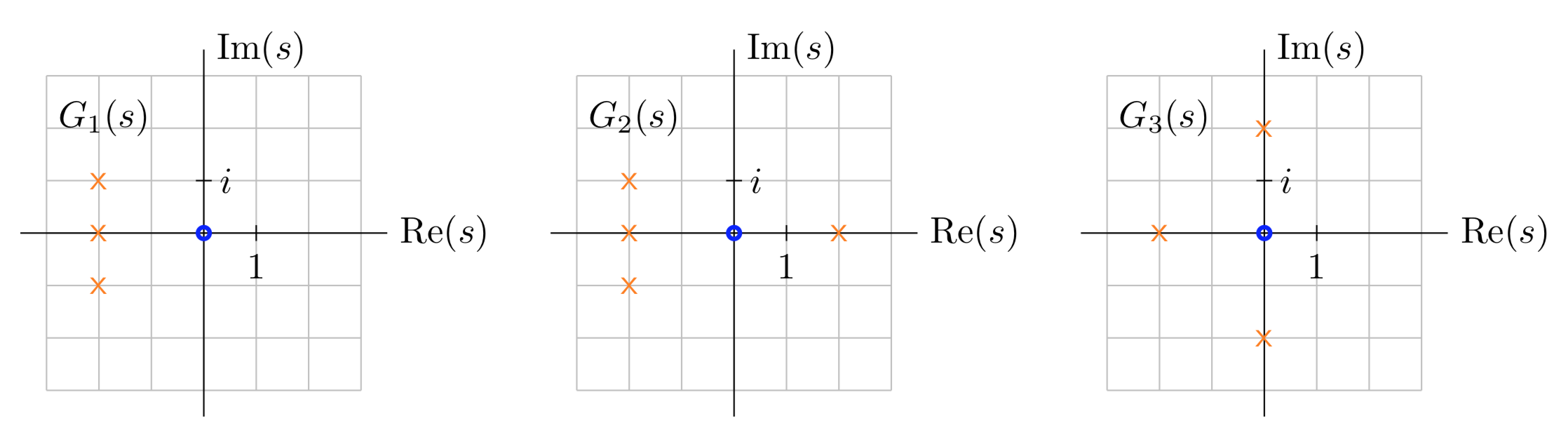
Pole-zero diagrams for the three systems.
bit about stability
This is just to give you a little physical orientation. Given our definition of stability above, we could, in principle, discuss stability without the slightest idea what it means for physical systems.
The poles of \(G(s)\) correspond to what are called modes of the system. A simple pole at \(s_1\) corresponds to a mode \(y_1 (t) = e^{s_1 t}\). The system is stable if the modes all decay to 0, i.e. if the poles are all in the left half-plane.
Physically the modes tell us the behavior of the system when the input signal is 0, but there are initial conditions. A pole with positive real part would correspond to a mode that goes to infinity as \(t\) grows. It is certainly reasonable to call a system that does this in response to a zero signal (often called ‘no input’) unstable.
To connect this to 18.03: if the system is modeled by a differential equation, the modes correspond to the homogeneous solutions \(y(t) = e^{st}\), where \(s\) is a root of the characteristic equation. In 18.03 we called the system stable if every homogeneous solution decayed to 0. That is, if the unforced system always settled down to equilibrium.
Closed loop systems
If the system with system function \(G(s)\) is unstable it can sometimes be stabilized by what is called a negative feedback loop. The new system is called a closed loop system. Its system function is given by Black's formula
\[G_{CL} (s) = \dfrac{G(s)}{1 + kG(s)}, \nonumber \]
where \(k\) is called the feedback factor. We will just accept this formula. Any class or book on control theory will derive it for you.
In this context \(G(s)\) is called the open loop system function.
Since \(G_{CL}\) is a system function, we can ask if the system is stable.
The poles of the closed loop system function \(G_{CL} (s)\) given in Equation 12.3.2 are the zeros of \(1 + kG(s)\).
- Proof
-
Looking at Equation 12.3.2, there are two possible sources of poles for \(G_{CL}\).
- The zeros of the denominator \(1 + k G\). The theorem recognizes these.
- The poles of \(G\). Since \(G\) is in both the numerator and denominator of \(G_{CL}\) it should be clear that the poles cancel. We can show this formally using Laurent series. If \(G\) has a pole of order \(n\) at \(s_0\) then
\[G(s) = \dfrac{1}{(s - s_0)^n} (b_n + b_{n - 1} (s - s_0) + \ ... a_0 (s - s_0)^n + a_1 (s - s_0)^{n + 1} + \ ...), \nonumber \]
where \(b_n \ne 0\). So,
\[\begin{array} {rcl} {G_{CL} (s)} & = & {\dfrac{\dfrac{1}{(s - s_0)^n} (b_n + b_{n - 1} (s - s_0) + \ ... a_0 (s - s_0)^n + \ ...)}{1 + \dfrac{k}{(s - s_0)^n} (b_n + b_{n - 1} (s - s_0) + \ ... a_0 (s - s_0)^n + \ ...)}} \\ { } & = & {\dfrac{(b_n + b_{n - 1} (s - s_0) + \ ... a_0 (s - s_0)^n + \ ...)}{(s - s_0)^n + k (b_n + b_{n - 1} (s - s_0) + \ ... a_0 (s - s_0)^n + \ ...)}} \end{array} \nonumber \]
which is clearly analytic at \(s_0\). (At \(s_0\) it equals \(b_n/(kb_n) = 1/k\).)
Set the feedback factor \(k = 1\). Assume \(a\) is real, for what values of \(a\) is the open loop system \(G(s) = \dfrac{1}{s + a}\) stable? For what values of \(a\) is the corresponding closed loop system \(G_{CL} (s)\) stable?
(There is no particular reason that \(a\) needs to be real in this example. But in physical systems, complex poles will tend to come in conjugate pairs.)
Solution
\(G(s)\) has one pole at \(s = -a\). Thus, it is stable when the pole is in the left half-plane, i.e. for \(a > 0\).
The closed loop system function is
\[G_{CL} (s) = \dfrac{1/(s + a)}{1 + 1/(s + a)} = \dfrac{1}{s + a + 1}. \nonumber \]
This has a pole at \(s = -a - 1\), so it's stable if \(a > -1\). The feedback loop has stabilized the unstable open loop systems with \(-1 < a \le 0\). (Actually, for \(a = 0\) the open loop is marginally stable, but it is fully stabilized by the closed loop.)
The algebra involved in canceling the \(s + a\) term in the denominators is exactly the cancellation that makes the poles of \(G\) removable singularities in \(G_{CL}\).
Suppose \(G(s) = \dfrac{s + 1}{s - 1}\). Is the open loop system stable? Is the closed loop system stable when \(k = 2\).
Solution
\(G(s)\) has a pole in the right half-plane, so the open loop system is not stable. The closed loop system function is
\[G_{CL} (s) = \dfrac{G}{1 + kG} = \dfrac{(s + 1)/(s - 1)}{1 + 2(s + 1)/(s - 1)} = \dfrac{s + 1}{3s + 1}. \nonumber \]
The only pole is at \(s = -1/3\), so the closed loop system is stable. This is a case where feedback stabilized an unstable system.
\(G(s) = \dfrac{s - 1}{s + 1}\). Is the open loop system stable? Is the closed loop system stable when \(k = 2\).
Solution
The only plot of \(G(s)\) is in the left half-plane, so the open loop system is stable. The closed loop system function is
\[G_{CL} (s) = \dfrac{G}{1 + kG} = \dfrac{(s - 1)/(s + 1)}{1 + 2(s - 1)/(s + 1)} = \dfrac{s - 1}{3s - 1}. \nonumber \]
This has one pole at \(s = 1/3\), so the closed loop system is unstable. This is a case where feedback destabilized a stable system. It can happen!
Nyquist Plots
For the Nyquist plot and criterion the curve \(\gamma\) will always be the imaginary \(s\)-axis. That is
\[s = \gamma (\omega) = i \omega, \text{ where } -\infty < \omega < \infty. \nonumber \]
For a system \(G(s)\) and a feedback factor \(k\), the Nyquist plot is the plot of the curve
\[w = k G \circ \gamma (\omega) = kG(i \omega). \nonumber \]
That is, the Nyquist plot is the image of the imaginary axis under the map \(w = kG(s)\).
In \(\gamma (\omega)\) the variable is a greek omega and in \(w = G \circ \gamma\) we have a double-u.
Let \(G(s) = \dfrac{1}{s + 1}\). Draw the Nyquist plot with \(k = 1\).
Solution
In the case \(G(s)\) is a fractional linear transformation, so we know it maps the imaginary axis to a circle. It is easy to check it is the circle through the origin with center \(w = 1/2\). You can also check that it is traversed clockwise.
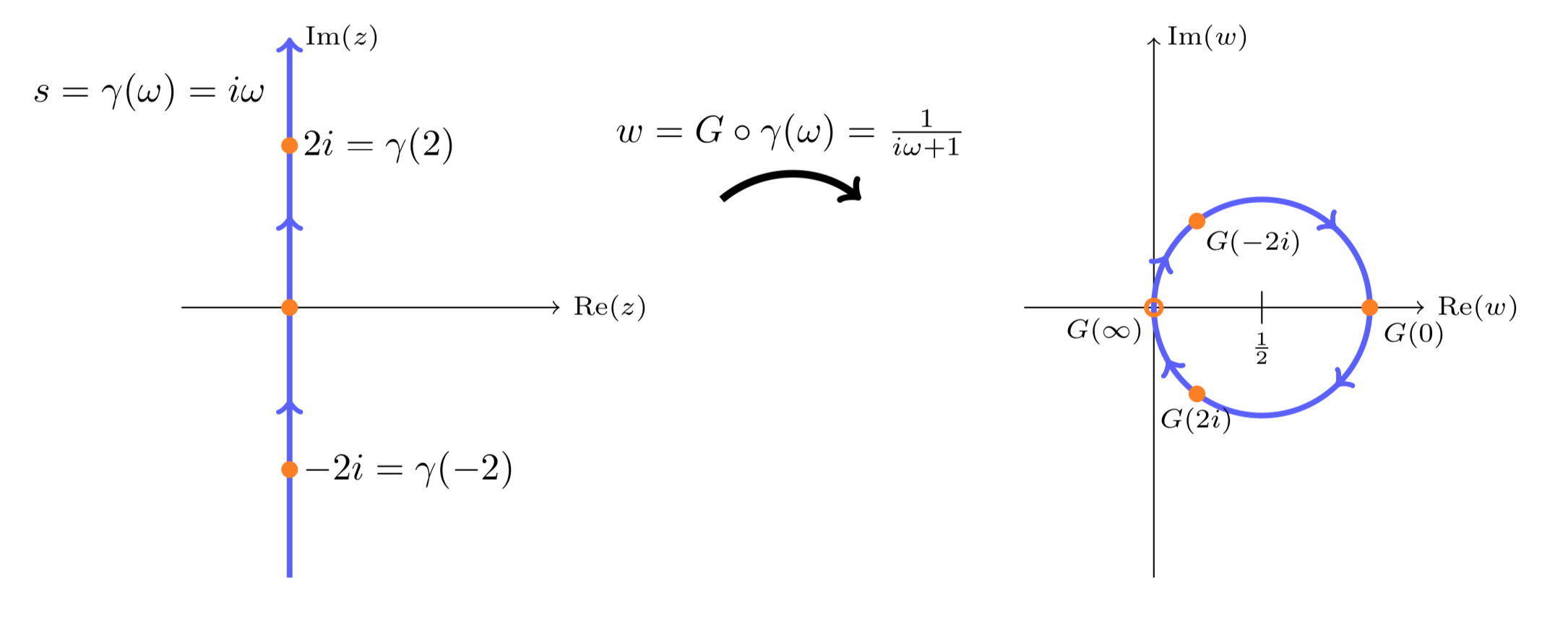
Nyquist plot of \(G(s) = 1/(s + 1)\), with \(k = 1\).
Take \(G(s)\) from the previous example. Describe the Nyquist plot with gain factor \(k = 2\).
Solution
The Nyquist plot is the graph of \(kG(i \omega)\). The factor \(k = 2\) will scale the circle in the previous example by 2. That is, the Nyquist plot is the circle through the origin with center \(w = 1\).
In general, the feedback factor will just scale the Nyquist plot.
Nyquist Criterion
The Nyquist criterion gives a graphical method for checking the stability of the closed loop system.
Suppose that \(G(s)\) has a finite number of zeros and poles in the right half-plane. Also suppose that \(G(s)\) decays to 0 as \(s\) goes to infinity. Then the closed loop system with feedback factor \(k\) is stable if and only if the winding number of the Nyquist plot around \(w = -1\) equals the number of poles of \(G(s)\) in the right half-plane.
More briefly,
\[G_{CL} (s) \text{ is stable } \Leftrightarrow \text{ Ind} (kG \circ \gamma, -1) = P_{G, RHP} \nonumber \]
Here, \(\gamma\) is the imaginary \(s\)-axis and \(P_{G, RHP}\) is the number o poles of the original open loop system function \(G(s)\) in the right half-plane.
- Proof
-
\(G_{CL}\) is stable exactly when all its poles are in the left half-plane. Now, recall that the poles of \(G_{CL}\) are exactly the zeros of \(1 + k G\). So, stability of \(G_{CL}\) is exactly the condition that the number of zeros of \(1 + kG\) in the right half-plane is 0.
Let’s work with a familiar contour.
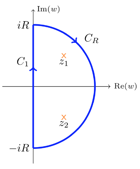
Let \(\gamma_R = C_1 + C_R\). Note that \(\gamma_R\) is traversed in the \(clockwise\) direction. Choose \(R\) large enough that the (finite number) of poles and zeros of \(G\) in the right half-plane are all inside \(\gamma_R\). Now we can apply Equation 12.2.4 in the corollary to the argument principle to \(kG(s)\) and \(\gamma\) to get
\[-\text{Ind} (kG \circ \gamma_R, -1) = Z_{1 + kG, \gamma_R} - P_{G, \gamma_R} \nonumber \]
(The minus sign is because of the clockwise direction of the curve.) Thus, for all large \(R\)
\[\text{the system is stable } \Leftrightarrow \ Z_{1 + kG, \gamma_R} = 0 \ \Leftrightarow \ \text{ Ind} (kG \circ \gamma_R, -1) = P_{G, \gamma_R} \nonumber \]
Finally, we can let \(R\) go to infinity. The assumption that \(G(s)\) decays 0 to as \(s\) goes to \(\infty\) implies that in the limit, the entire curve \(kG \circ C_R\) becomes a single point at the origin. So in the limit \(kG \circ \gamma_R\) becomes \(kG \circ \gamma\). \(\text{QED}\)
Examples using the Nyquist Plot mathlet
The Nyquist criterion is a visual method which requires some way of producing the Nyquist plot. For this we will use one of the MIT Mathlets (slightly modified for our purposes). Open the Nyquist Plot applet at
http://web.mit.edu/jorloff/www/jmoapplets/nyquist/nyquistCrit.html
Play with the applet, read the help.
Now refresh the browser to restore the applet to its original state. Check the \(Formula\) box. The formula is an easy way to read off the values of the poles and zeros of \(G(s)\). In its original state, applet should have a zero at \(s = 1\) and poles at \(s = 0.33 \pm 1.75 i\).
The left hand graph is the pole-zero diagram. The right hand graph is the Nyquist plot.
To get a feel for the Nyquist plot. Look at the pole diagram and use the mouse to drag the yellow point up and down the imaginary axis. Its image under \(kG(s)\) will trace out the Nyquis plot.
Notice that when the yellow dot is at either end of the axis its image on the Nyquist plot is close to 0.
Refresh the page, to put the zero and poles back to their original state. There are two poles in the right half-plane, so the open loop system \(G(s)\) is unstable. With \(k =1\), what is the winding number of the Nyquist plot around -1? Is the closed loop system stable?
Solution
The curve winds twice around -1 in the counterclockwise direction, so the winding number \(\text{Ind} (kG \circ \gamma, -1) = 2\). Since the number of poles of \(G\) in the right half-plane is the same as this winding number, the closed loop system is stable.
With the same poles and zeros, move the \(k\) slider and determine what range of \(k\) makes the closed loop system stable.
Solution
When \(k\) is small the Nyquist plot has winding number 0 around -1. For these values of \(k\), \(G_{CL}\) is unstable. As \(k\) increases, somewhere between \(k = 0.65\) and \(k = 0.7\) the winding number jumps from 0 to 2 and the closed loop system becomes stable. This continues until \(k\) is between 3.10 and 3.20, at which point the winding number becomes 1 and \(G_{CL}\) becomes unstable.
Answer: The closed loop system is stable for \(k\) (roughly) between 0.7 and 3.10.
In the previous problem could you determine analytically the range of \(k\) where \(G_{CL} (s)\) is stable?
Solution
Yes! This is possible for small systems. It is more challenging for higher order systems, but there are methods that don’t require computing the poles. In this case, we have
\[G_{CL} (s) = \dfrac{G(s)}{1 + kG(s)} = \dfrac{\dfrac{s - 1}{(s - 0.33)^2 + 1.75^2}}{1 + \dfrac{k(s - 1)}{(s - 0.33)^2 + 1.75^2}} = \dfrac{s - 1}{(s - 0.33)^2 + 1.75^2 + k(s - 1)} \nonumber \]
So the poles are the roots of
\[(s - 0.33)^2 + 1.75^2 + k(s - 1) = s^2 + (k - 0.66)s + 0.33^2 + 1.75^2 - k \nonumber \]
For a quadratic with positive coefficients the roots both have negative real part. This happens when
\[0.66 < k < 0.33^2 + 1.75^2 \approx 3.17. \nonumber \]
What happens when \(k\) goes to 0.
Solution
As \(k\) goes to 0, the Nyquist plot shrinks to a single point at the origin. In this case the winding number around -1 is 0 and the Nyquist criterion says the closed loop system is stable if and only if the open loop system is stable.
This should make sense, since with \(k = 0\),
\[G_{CL} = \dfrac{G}{1 + kG} = G. \nonumber \]
Make a system with the following zeros and poles:
- A pair of zeros at \(0.6 \pm 0.75i\).
- A pair of poles at \(-0.5 \pm 2.5i\).
- A single pole at 0.25.
Is the corresponding closed loop system stable when \(k = 6\)?
Solution
The answer is no, \(G_{CL}\) is not stable. \(G\) has one pole in the right half plane. The mathlet shows the Nyquist plot winds once around \(w = -1\) in the \(clockwise\) direction. So the winding number is -1, which does not equal the number of poles of \(G\) in the right half-plane.
If we set \(k = 3\), the closed loop system is stable.