
3.3: Intervals in Eⁿ
- Page ID
- 19037

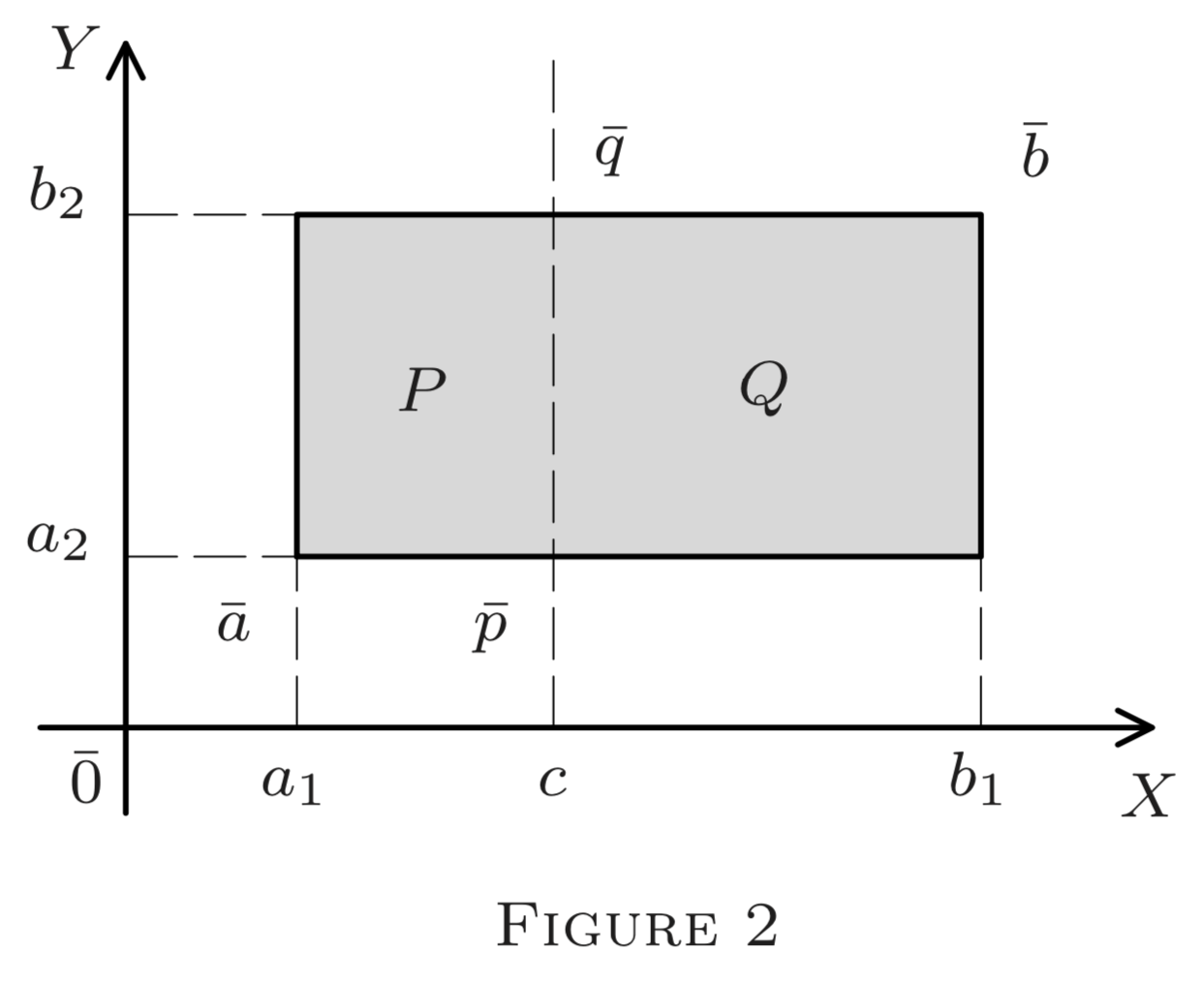
Consider the rectangle in \(E^{2}\) shown in Figure 2. Its interior (without the perimeter consists of all points \((x, y) \in E^{2}\) such that
\[a_{1}<x<b_{1}\text{ and } a_{2}<y<b_{2};\]
i.e.,
\[x \in\left(a_{1}, b_{1}\right)\text{ and } y \in\left(a_{2}, b_{2}\right).\]
Thus it is the Cartesian product of two line intervals, \(\left(a_{1}, b_{1}\right)\) and \(\left(a_{2}, b_{2}\right) .\) To include also all or some sides, we would have to replace open intervals by closed, half-closed, or half-open ones. Similarly, Cartesian products of three line intervals yield rectangular parallelepipeds in \(E^{3} .\) We call such sets in \(E^{n}\) intervals.
1. By an interval in \(E^{n}\) we mean the Cartesian product of any \(n\) intervals \(\quad\) in \(E^{1}\) (some may be open, some closed or half-open, etc.).
2. In particular, given
\[\overline{a}=\left(a_{1}, \ldots, a_{n}\right)\text{ and } \overline{b}=\left(b_{1}, \ldots, b_{n}\right)\]
with
\[a_{k} \leq b_{k}, \quad k=1,2, \ldots, n,\]
we define the open interval \((\overline{a}, \overline{b}),\) the closed interval \([\overline{a}, \overline{b}],\) the half-open interval \((\overline{a}, \overline{b}],\) and the half-closed interval \([\overline{a}, \overline{b})\) as follows:
\[\begin{aligned}(\overline{a}, \overline{b}) &=\left\{\overline{x} | a_{k}<x_{k}<b_{k}, k=1,2, \ldots, n\right\} \\ &=\left(a_{1}, b_{1}\right) \times\left(a_{2}, b_{2}\right) \times \cdots \times\left(a_{n}, b_{n}\right) \\ [\overline{a}, \overline{b}] &=\left\{\overline{x} | a_{k} \leq x_{k} \leq b_{k}, k=1,2, \ldots, n\right\} \\ &=\left[a_{1}, b_{1}\right] \times\left[a_{2}, b_{2}\right] \times \cdots \times\left[a_{n}, b_{n}\right] \\ (\overline{a}, \overline{b}] &=\left\{\overline{x} | a_{k}<x_{k} \leq b_{k}, k=1,2, \ldots, n\right\} \\ &=\left(a_{1}, b_{1}\right] \times\left(a_{2}, b_{2}\right] \times \cdots \times\left(a_{n}, b_{n}\right] \\ [a, b) &=\left\{\overline{x} | a_{k} \leq x_{k}<b_{k}, k=1,2, \ldots, n\right\} \\ &=\left[a_{1}, b_{1}\right) \times\left[a_{2}, b_{2}\right) \times \cdots \times\left[a_{n}, b_{n}\right) \end{aligned}\]
In all cases, \(\overline{a}\) and \(\overline{b}\) are called the endpoints of the interval. Their distance
\[\rho(\overline{a}, \overline{b})=|\overline{b}-\overline{a}|\]
is called its diagonal. The \(n\) differences
\[b_{k}-a_{k}=\ell_{k} \quad(k=1, \ldots, n)\]
are called its \(n\) edge-lengths. Their product
\[\prod_{k=1}^{n} \ell_{k}=\prod_{k=1}^{n}\left(b_{k}-a_{k}\right)\]
is called the volume of the interval (in \(E^{2}\) it is its area, in \(E^{1}\) its length) .\) The point
\[\overline{c}=\frac{1}{2}(\overline{a}+\overline{b})\]
is called its center or midpoint. The set difference
\[[\overline{a}, \overline{b}]-(\overline{a}, \overline{b})\]
is called the boundary of any interval with endpoints \(\overline{a}\) and \(\vec{b} ;\) it consists of 2\(n\) "faces" defined in a natural manner. (How?)
We often denote intervals by single letters, e.g.. \(A=(\overline{a}, \overline{b}),\) and write \(d A\) for "diagonal of \(A^{\prime \prime}\) and \(v A\) or vol \(A\) for "volume of \(A . "\) If all edge-lengths \(b_{k}-a_{k}\) are equal, \(A\) is called a cube (in \(E^{2},\) a square). The interval \(A\) is said to be degenerate iff \(b_{k}=a_{k}\) for some \(k,\) in which case, clearly,
\[\operatorname{vol} A=\prod_{k=1}^{n}\left(b_{k}-a_{k}\right)=0.\]
Note 1. We have \(\overline{x} \in(\overline{a}, \overline{b})\) iff the inequalities \(a_{k}<x_{k}<b_{k}\) hold simultaneously for all \(k .\) This is impossible if \(a_{k}=b_{k}\) for some \(k ;\) similarly for the inequalities \(a_{k}<x_{k} \leq b_{k}\) or \(a_{k} \leq x_{k}<b_{k}\). Thus a degenerate interval is empty, unless it is closed (in which case it contains \(\overline{a}\) and \(\overline{b}\) at least).
Note 2. In any interval \(A\),
\[d A=\rho(\overline{a}, \overline{b})=\sqrt{\sum_{k=1}^{n}\left(b_{k}-a_{k}\right)^{2}}=\sqrt{\sum_{k=1}^{n} \ell_{k}^{2}}.\]
In \(E^{2},\) we can split an interval \(A\) into two subintervals \(P\) and \(Q\) by drawing a line (see Figure 2\() .\) In \(E^{3},\) this is done by a plane orthogonal to one of the axes of the form \(x_{k}=c\left(\) see §§4-6, Note 2\(),\) with \(a_{k}<c<b_{k} .\) In particular, if \right. \(c=\frac{1}{2}\left(a_{k}+b_{k}\right),\) the plane bisects the \(k\) th edge of \(A ;\) and so the \(k\) th edge-length of \(P(\) and \(Q)\) equals \(\frac{1}{2} \ell_{k}=\frac{1}{2}\left(b_{k}-a_{k}\right) .\) If \(A\) is closed, so is \(P\) or \(Q,\) depending on our choice. (We may include the "partition" \(x_{k}=c\) in \(P\) or \(Q . )^{1}\)
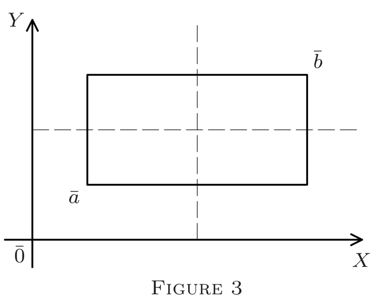
Now, successively draw \(n\) planes \(x_{k}=c_{k}, \quad c_{k}=\frac{1}{2}\left(a_{k}+b_{k}\right), \quad k=1,2, \ldots, n .\) The first plane bisects \(\ell_{j}\) leaving the other edges of \(A \mathrm{un}-\) changed. The resulting two subintervals \(P\) and \(Q\) then are cut by the plane \(x_{2}=c_{2},\) bisecting the second edge in each of them. Thus we get four subintervals (see Figure 3 for \(E^{2}\). Each successive plane doubles the number of subintervals. After \(n\) steps, we thus obtain \(2^{n}\) disjoint intervals, with all edges \(\ell_{k}\) bisected. Thus by Note \(2,\) the diagonal of each of them is
\[\sqrt{\sum_{k=1}^{n}\left(\frac{1}{2} \ell_{k}\right)^{2}}=\frac{1}{2} \sqrt{\sum_{k=1}^{n} \ell_{k}^{2}}=\frac{1}{2} d A.\]
Note 3. If \(A\) is closed then, as noted above, we can make any one (but only one \()\) of the \(2^{n}\) subintervals closed by properly manipulating each step.
The proof of the following simple corollaries is left to the reader.
No distance between two points of an interval \(A\) exceeds \(d A,\) its diagonal. That is, \((\forall \overline{x}, \overline{y} \in A) \rho(\overline{x}, \overline{y}) \leq d A\)
If an interval \(A\) contains \(\overline{p}\) and \(\overline{q},\) then also \(L[\overline{p}, \overline{q}] \subseteq A\).
Every nondegenerate interval in \(E^{n}\) contains rational points, i.e., points whose coordinates are all rational.
(Hint: Use the density of rationals in \(E^{1}\) for each coordinate separately.)