5.2: Derivatives of Extended-Real Functions

For a while (in §§2 and 3), we limit ourselves to extended-real functions. Below, 𝑓 and 𝑔 are real or extended real (f, 𝑔 :𝐸1 →𝐸∗). We assume, however, that they are not constantly infinite on any interval (𝑎,𝑏),𝑎 <𝑏.

Lemma 5.2.1

If 𝑓′⁡(𝑝) >0 at some 𝑝 ∈𝐸1, then

𝑥<𝑝<𝑦(5.2.1)

implies

𝑓⁡(𝑥)<𝑓⁡(𝑝)<𝑓⁡(𝑦)(5.2.2)

for all 𝑥,𝑦 in a sufficiently small globe 𝐺𝑝⁡(𝛿) =(𝑝 −𝛿,𝑝 +𝛿).

Similarly, if 𝑓′⁡(𝑝) <0, then 𝑥 <𝑝 <𝑦 implies 𝑓⁡(𝑥) >𝑓⁡(𝑝) >𝑓⁡(𝑦) for 𝑥,𝑦 in some 𝐺𝑝⁡(𝛿).

Proof

If 𝑓′⁡(𝑝) >0, the "0" case in Definition 1 of §1, is excluded, so

𝑓′⁡(𝑝)=lim𝑥→𝑝⁡Δ⁢𝑓Δ⁢𝑥>0.(5.2.3)

Hence we must also have Δ⁢𝑓⁡/Δ⁢𝑥 >0 for 𝑥 in some 𝐺𝑝⁡(𝛿).

It follows that Δ⁢𝑓 and Δ⁢𝑥 have the same sign in 𝐺𝑝⁡(𝛿); i.e.,

𝑓⁡(𝑥)−𝑓⁡(𝑝)>0 if 𝑥>𝑝 and 𝑓⁡(𝑥)−𝑓⁡(𝑝)<0 if 𝑥<𝑝.(5.2.4)

(This implies 𝑓⁡(𝑝) ≠±∞. Why? Hence

𝑥<𝑝<𝑦⟹𝑓⁡(𝑥)<𝑓⁡(𝑝)<𝑓⁡(𝑦),(5.2.5)

as claimed; similarly in case 𝑓′⁡(𝑝) <0. ◻

Corollary 5.2.1

If 𝑓⁡(𝑝) is the maximum or minimum value of 𝑓⁡(𝑥) for 𝑥 in some 𝐺𝑝⁡(𝛿), then 𝑓′⁡(𝑝) =0; i.e., 𝑓 has a zero derivative, or none at all, at 𝑝.

For, by Lemma 1, 𝑓′⁡(𝑝) ≠0 excludes a maximum or minimum at 𝑝. (Why?)

Note 1. Thus 𝑓′⁡(𝑝) =0 is a necessary condition for a local maximum or minimum at 𝑝. It is insufficient, however. For example, if 𝑓⁡(𝑥) =𝑥3,𝑓 has no maxima or minima at all, yet 𝑓′⁡(0) =0. For sufficient conditions, see §6.

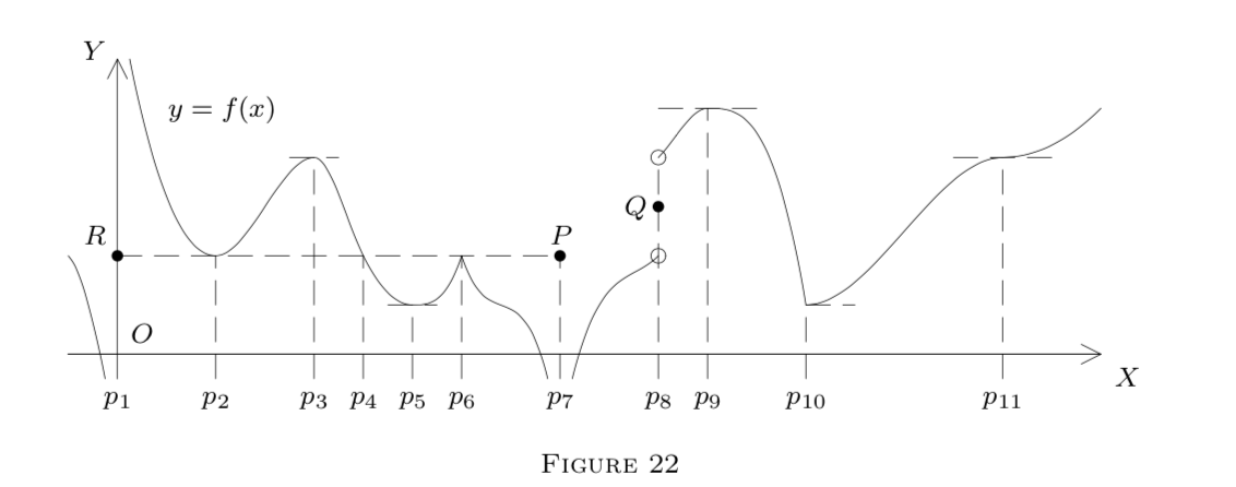
Figure 22 illustrates these facts at the points 𝑝2,𝑝3,…,𝑝11. Note that in Figure 22, the isolated points 𝑃,𝑄,𝑅 belong to the graph.

Geometrically, 𝑓′⁡(𝑝) =0 means that the tangent at 𝑝 is horizontal, or that a two-sided tangent does not exist at 𝑝.

Theorem 5.2.1

Let 𝑓 :𝐸1 →𝐸∗ be relatively continuous on an interval [𝑎,𝑏], with 𝑓′ ≠0 on (𝑎,𝑏). Then 𝑓 is strictly monotone on [𝑎,𝑏], and 𝑓′ is signconstant there (possibly 0 at a and b), with 𝑓′ ≥0 if 𝑓 ↑, and 𝑓′ ≤0 if 𝑓 ↓.

Proof

By Theorem 2 of Chapter 4, §8, 𝑓 attains a least value 𝑚, and a largest value 𝑀, at some points of [𝑎,𝑏]. However, neither can occur at an interior point 𝑝 ∈(𝑎,𝑏), for, by Corollary 1, this would imply 𝑓′⁡(𝑝) =0, contrary to our assumption.

Thus 𝑀 =𝑓⁡(𝑎) or 𝑀 =𝑓⁡(𝑏); for the moment we assume 𝑀 =𝑓⁡(𝑏) and 𝑚 =𝑓⁡(𝑎). We must have 𝑚 <𝑀, for 𝑚 =𝑀 would make 𝑓 constant on [𝑎,𝑏], implying 𝑓′ =0. Thus 𝑚 =𝑓⁡(𝑎) <𝑓⁡(𝑏) =𝑀.

Now let 𝑎 ≤𝑥 <𝑦 ≤𝑏. Applying the previous argument to each of the intervals [𝑎,𝑥],[𝑎,𝑦],[𝑥,𝑦], and [𝑥,𝑏] (now using that 𝑚 =𝑓⁡(𝑎) <𝑓⁡(𝑏) =𝑀), we find that

𝑓⁡(𝑎)≤𝑓⁡(𝑥)<𝑓⁡(𝑦)≤𝑓⁡(𝑏). (Why?) (5.2.6)

Thus 𝑎 ≤𝑥 <𝑦 ≤𝑏 implies 𝑓⁡(𝑥) <𝑓⁡(𝑦); i.e., 𝑓 increases on [𝑎,𝑏]. Hence 𝑓′ cannot be negative at any 𝑝 ∈[𝑎,𝑏], for, otherwise, by Lemma 1, 𝑓 would decrease at 𝑝. Thus 𝑓′ ≥0 on [𝑎,𝑏].

In the case 𝑀 =𝑓⁡(𝑎) >𝑓⁡(𝑏) =𝑚, we would obtain 𝑓′ ≤0. ◻

Caution: The function 𝑓 may increase or decrease at 𝑝 even if 𝑓′⁡(𝑝) =0.
See Note 1.

Corollary 5.2.2 (Rolle's theorem)

If : 𝐸1 →𝐸∗ is relatively continuous on [𝑎,𝑏] and if 𝑓⁡(𝑎) =𝑓⁡(𝑏), then 𝑓′⁡(𝑝) =0 for at least one interior point 𝑝 ∈(𝑎,𝑏).

For, if 𝑓′ ≠0 on all of (𝑎,𝑏), then by Theorem 1, 𝑓 would be strictly monotone on [𝑎,𝑏], so the equality 𝑓⁡(𝑎) =𝑓⁡(𝑏) would be impossible.

Figure 22 illustrates this on the intervals [𝑝2,𝑝4] and [𝑝4,𝑝6], with 𝑓′⁡(𝑝3) = 𝑓′⁡(𝑝5) =0. A discontinuity at 0 causes an apparent failure on [0,𝑝2].

Note 2. Theorem 1 and Corollary 2 hold even if 𝑓⁡(𝑎) and 𝑓⁡(𝑏) are infinite, if continuity is interpreted in the sense of the metric 𝜌′ of Problem 5 in Chapter 3, §11. (Weierstrass' Theorem 2 of Chapter 4, §8 applies to (𝐸∗,𝜌′), with the same proof.)

Theorem 5.2.2 (Cauchy's law of the mean)

Let the functions 𝑓,𝑔 :𝐸1 →𝐸∗ be relatively continuous and finite on [𝑎,𝑏] and have derivatives on (𝑎,𝑏), with 𝑓′ and 𝑔′ never both infinite at the same point 𝑝 ∈(𝑎,𝑏). Then

𝑔′⁡(𝑞)⁢[𝑓⁡(𝑏)−𝑓⁡(𝑎)]=𝑓′⁡(𝑞)⁢[𝑔⁡(𝑏)−𝑔⁡(𝑎)] for at least one 𝑞∈(𝑎,𝑏).(5.2.7)

Proof

Let 𝐴 =𝑓⁡(𝑏) −𝑓⁡(𝑎) and 𝐵 =𝑔⁡(𝑏) −𝑔⁡(𝑎). We must show that 𝐴⁢𝑔′⁡(𝑞) =𝐵⁢𝑓′⁡(𝑞) for some 𝑞 ∈(𝑎,𝑏). For this purpose, consider the function ℎ =𝐴⁢𝑔 −𝐵⁢𝑓. It is relatively continuous and finite on [𝑎,𝑏], as are 𝑔 and 𝑓. Also,

ℎ⁡(𝑎)=𝑓⁡(𝑏)⁢𝑔⁡(𝑎)−𝑔⁡(𝑏)⁢𝑓⁡(𝑎)=ℎ⁡(𝑏). (Verify!) (5.2.8)

Thus by Corollary 2, ℎ′⁡(𝑞) =0 for some 𝑞 ∈(𝑎,𝑏). Here, by Theorem 4 of §1, ℎ′ =(𝐴⁢𝑔−𝐵⁢𝑓)′ =𝐴⁢𝑔′ −𝐵⁢𝑓′. (This is legitimate, for, by assumption, 𝑓′ and 𝑔′ never both become infinite, so no indeterminate limits occur.) Thus ℎ′⁡(𝑞) =𝐴⁢𝑔′⁡(𝑞) −𝐵⁢𝑓′⁡(𝑞) =0, and (1) follows. ◻

Corollary 5.2.3 (Lagrange's law of the mean)

If 𝑓 :𝐸1 →𝐸1 is relatively continuous on [𝑎,𝑏] with a derivative on (𝑎,𝑏), then

𝑓⁡(𝑏)−𝑓⁡(𝑎)=𝑓′⁡(𝑞)⁢(𝑏−𝑎) for at least one 𝑞∈(𝑎,𝑏).(5.2.9)

Proof

Take 𝑔⁡(𝑥) =𝑥 in Theorem 2, so 𝑔′ =1 on 𝐸1.◻

Note 3. Geometrically,

𝑓⁡(𝑏)−𝑓⁡(𝑎)𝑏−𝑎(5.2.10)

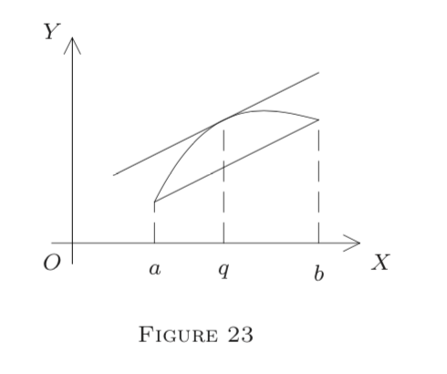
is the slope of the secant through (𝑎,𝑓⁡(𝑎)) and (𝑏,𝑓⁡(𝑏)), and 𝑓′⁡(𝑞) is the slope of the tangent line at 𝑞. Thus Corollary 3 states that the secant is parallel to the tangent at some intermediate point 𝑞; see Figure 23. Theorem 2 states the same for curves given parametrically: 𝑥 =𝑓⁡(𝑡),𝑦 =𝑔⁡(𝑡).

Corollary 5.2.4

Let 𝑓 be as in Corollary 3. Then

(i) 𝑓 is constant on [𝑎,𝑏] iff 𝑓′ =0 on (𝑎,𝑏);

(ii) 𝑓 ↑ on [𝑎,𝑏] iff 𝑓′ ≥0 on (𝑎,𝑏); and

(iii) 𝑓 ↓ on [𝑎,𝑏] iff 𝑓′ ≤0 on (𝑎,𝑏).

Proof

Let 𝑓′ =0 on (𝑎,𝑏). If 𝑎 ≤𝑥 ≤𝑦 ≤𝑏, apply Corollary 3 to the interval [𝑥,𝑦] to obtain

𝑓⁡(𝑦)−𝑓⁡(𝑥)=𝑓′⁡(𝑞)⁢(𝑦−𝑥) for some 𝑞∈(𝑎,𝑏) and 𝑓′⁡(𝑞)=0.(5.2.11)

Thus 𝑓⁡(𝑦) −𝑓⁡(𝑥) =0 for 𝑥,𝑦 ∈[𝑎,𝑏], so 𝑓 is constant.

The rest is left to the reader. ◻

Theorem 5.2.3 (inverse functions)

Let 𝑓 :𝐸1 →𝐸1 be relatively continuous and strictly monotone on an interval 𝐼 ⊆𝐸1. Let 𝑓′⁡(𝑝) ≠0 at some interior point 𝑝 ∈𝐼. Then the inverse function 𝑔 =𝑓−1 (with 𝑓 restricted to 𝐼) has a derivative at 𝑞 =𝑓⁡(𝑝), and

𝑔′⁡(𝑞)=1𝑓′⁡(𝑝).(5.2.12)

(If 𝑓′⁡(𝑝) =±∞, then 𝑔′⁡(𝑞) =0.)

Proof

By Theorem 3 of Chapter 4, §9, 𝑔 =𝑓−1 is strictly monotone and relatively continuous on 𝑓⁡[𝐼], itself an interval. If 𝑝 is interior to 𝐼, then 𝑞 =𝑓⁡(𝑝) is interior to 𝑓⁡[𝐼]. (Why?)

Now if 𝑦 ∈𝑓⁡[𝐼], we set

Δ⁢𝑔=𝑔⁡(𝑦)−𝑔⁡(𝑞),Δ⁢𝑦=𝑦−𝑞,𝑥=𝑓−1⁡(𝑦)=𝑔⁡(𝑦), and 𝑓⁡(𝑥)=𝑦(5.2.13)

and obtain

Δ⁢𝑔Δ⁢𝑦=𝑔⁡(𝑦)−𝑔⁡(𝑞)𝑦−𝑞=𝑥−𝑝𝑓⁡(𝑥)−𝑓⁡(𝑝)=Δ⁢𝑥Δ⁢𝑓 for 𝑥≠𝑝.(5.2.14)

Now if 𝑦 →𝑞, the continuity of 𝑔 at 𝑞 yields 𝑔⁡(𝑦) →𝑔⁡(𝑞); i.e., 𝑥 →𝑝. Also, 𝑥 ≠𝑝 iff 𝑦 ≠𝑞, for 𝑓 and 𝑔 are one-to-one functions. Thus we may substitute 𝑦 =𝑓⁡(𝑥) or 𝑥 =𝑔⁡(𝑦) to get

𝑔′⁡(𝑞)=lim𝑦→𝑞⁡Δ⁢𝑔Δ⁢𝑦=lim𝑥→𝑝⁡Δ⁢𝑥Δ⁢𝑓=1lim𝑥→𝑝⁡(Δ⁢𝑓⁡/Δ⁢𝑥)=1𝑓′⁡(𝑝),(5.2.15)

where we use the convention 1∞ =0 if 𝑓′⁡(𝑝) =∞. ◻

Examples

(A) Let

𝑓⁡(𝑥)=log𝑎⁡|𝑥| with 𝑓⁡(0)=0.(5.2.16)

Let 𝑝 >0. Then (∀𝑥 >0)

Δ⁢𝑓=𝑓⁡(𝑥)−𝑓⁡(𝑝)=log𝑎⁡𝑥−log𝑎⁡𝑝=log𝑎⁡(𝑥/𝑝)=log𝑎⁡𝑝+(𝑥−𝑝)𝑝=log𝑎⁡(1+Δ⁢𝑥𝑝).(5.2.17)

Thus

Δ⁢𝑓Δ⁢𝑥=log𝑎⁡(1+Δ⁢𝑥𝑝)1/Δ⁢𝑥.(5.2.18)

Now let 𝑧 =Δ⁢𝑥/𝑝. (Why is this substitution admissible?) Then using the formula

lim𝑧→0⁡(1+𝑧)1/𝑧=𝑒 (see Chapter 4, §2, Example (C)) (5.2.19)

and the continuity of the log and power functions, we obtain

𝑓′⁡(𝑝)=lim𝑥→𝑝⁡Δ⁢𝑓Δ⁢𝑥=lim𝑧→0⁡log𝑎⁡[(1+𝑧)1/𝑧]1/𝑝=log𝑎⁡𝑒1/𝑝=1𝑝⁢log𝑎⁡𝑒.(5.2.20)

The same formula results also if 𝑝 <0, i.e., |𝑝| =−𝑝. At 𝑝 =0,𝑓 has one-sided derivatives (±∞) only (verify!), so 𝑓′⁡(0) =0 by Definition 1 in §1.

(B) The inverse of the log 𝑎 function is the exponential 𝑔 :𝐸1 →𝐸1, with

𝑔⁡(𝑦)=𝑎𝑦(𝑎>0,𝑎≠1).(5.2.21)

By Theorem 3, we have

(∀𝑞∈𝐸1)𝑔′⁡(𝑞)=1𝑓′⁡(𝑝),𝑝=𝑔⁡(𝑞)=𝑎𝑞.(5.2.22)

Thus

𝑔′⁡(𝑞)=11𝑝⁢log𝑎⁡𝑒=𝑝log𝑎⁡𝑒=𝑎𝑞log𝑎⁡𝑒.(5.2.23)

Symbolically,

(log𝑎⁡|𝑥|)′=1𝑥⁢log𝑎⁡𝑒⁡(𝑥≠0);(𝑎𝑥)′=𝑎𝑥log𝑎⁡𝑒=𝑎𝑥⁢ln⁡𝑎.(5.2.24)

In particular, if 𝑎 =𝑒, we have log𝑒⁡𝑎 =1 and log𝑎⁡𝑥 =ln⁡𝑥; hence

(ln⁡|𝑥|)′=1𝑥⁢(𝑥≠0) and (𝑒𝑥)′=𝑒𝑥(𝑥∈𝐸1).(5.2.25)

(C) The power function 𝑔 :(0,+∞) →𝐸1 is given by

𝑔⁡(𝑥)=𝑥𝑎=exp⁡(𝑎⋅ln⁡𝑥) for 𝑥>0 and fixed 𝑎∈𝐸1.(5.2.26)

By the chain rule (§1, Theorem 3), we obtain

𝑔′⁡(𝑥)=exp⁡(𝑎⋅ln⁡𝑥)⋅𝑎𝑥=𝑥𝑎⋅𝑎𝑥=𝑎⋅𝑥𝑎−1.(5.2.27)

Thus we have the symbolic formula

(𝑥𝑎)′=𝑎⋅𝑥𝑎−1 for 𝑥>0 and fixed 𝑎∈𝐸1.(5.2.28)

Theorem 5.2.4 (Darboux)

If 𝑓 :𝐸1 →𝐸∗ is relatively continuous and has a derivative on an interval I, then 𝑓′ has the Darboux property (Chapter 4, §9 ) on 𝐼.

Proof

Let 𝑝,𝑞 ∈𝐼 and 𝑓′⁡(𝑝) <𝑐 <𝑓′⁡(𝑞). Put 𝑔⁡(𝑥) =𝑓⁡(𝑥) −𝑐⁢𝑥. Assume 𝑔′ ≠0 on (𝑝,𝑞) and find a contradiction to Theorem 1. Details are left to the reader. ◻