6.7: Inverse and Implicit Functions. Open and Closed Maps

I. "If $f \in C D^{1}$ at $\vec{p},$ then $f$ resembles a linear map (namely $d f )$ at $\vec{p}."$ Pursuing this basic idea, we first make precise our notion of "$f \in C D^{1}$ at $\vec{p}$."

Definition 1

A map $f : E^{\prime} \rightarrow E$ is continuously differentiable, or of class $C D^{1}$ (written $f \in C D^{1}),$ at $\vec{p}$ iff the following statement is true:

$$\begin{array}{l}{\text { Given any } \varepsilon>0, \text { there is } \delta>0 \text { such that } f \text { is differentiable on the }} \\ {\text { globe } \overline{G}=\overline{G_{\vec{p}}(\delta)}, \text { with }} \\ {\qquad\|d f(\vec{x} ; \cdot)-d f(\vec{p} ; \cdot)\|<\varepsilon \text { for all } \vec{x} \in \overline{G}.}\end{array}$$

By Problem 10 in §5, this definition agrees with Definition 1 §5, but is no longer limited to the case $E^{\prime}=E^{n}\left(C^{n}\right).$ See also Problems 1 and 2 below.

We now obtain the following result.

Theorem $\PageIndex{1}$

Let $E^{\prime}$ and $E$ be complete. If $f : E^{\prime} \rightarrow E$ is of class $C D^{1}$ at $\vec{p}$ and if $d f(\vec{p} ; \cdot)$ is bijective (§6), then $f$ is one-to-one on some globe $\overline{G}=\overline{G_{\vec{p}}}(\delta).$

Thus $f$ "locally" resembles df $(\vec{p} ; \cdot)$ in this respect.

Proof

Set $\phi=d f(\vec{p} ; \cdot)$ and

$$\left\|\phi^{-1}\right\|=\frac{1}{\varepsilon}$$

(cf. Theorem 2 of §6).

By Definition 1, fix $\delta>0$ so that for $\vec{x} \in \overline{G}=\overline{G_{\vec{p}}(\delta)}$.

$$\|d f(\vec{x} ; \cdot)-\phi\|<\frac{1}{2} \varepsilon.$$

Then by Note 5 in §2,

$$(\forall \vec{x} \in \overline{G})\left(\forall \vec{u} \in E^{\prime}\right) \quad|d f(\vec{x} ; \vec{u})-\phi(\vec{u})| \leq \frac{1}{2} \varepsilon|\vec{u}|.$$

Now fix any $\vec{r}, \vec{s} \in \overline{G}, \vec{r} \neq \vec{s},$ and set $\vec{u}=\vec{r}-\vec{s} \neq 0.$ Again, by Note 5 in §2,

$$|\vec{u}|=\left|\phi^{-1}(\phi(\vec{u}))\right| \leq\left\|\phi^{-1}\right\||\phi(\vec{u})|=\frac{1}{\varepsilon}|\phi(\vec{u})|;$$

so

$$0<\varepsilon|\vec{u}| \leq|\phi(\vec{u})|.$$

By convexity, $\overline{G} \supseteq I=L[\vec{s}, \vec{r}],$ so (1) holds for $\vec{x} \in I, \vec{x}=\vec{s}+t \vec{u}, 0 \leq t \leq 1$.

Noting this, set

$$h(t)=f(\vec{s}+t \vec{u})-t \phi(\vec{u}), \quad t \in E^{1}.$$

Then for $0 \leq t \leq 1$,

$$\begin{aligned} h^{\prime}(t) &=D_{\vec{u}} f(\vec{s}+t \vec{u})-\phi(\vec{u}) \\ &=d f(\vec{s}+t \vec{u} ; \vec{u})-\phi(\vec{u}). \end{aligned}$$

(Verify!) Thus by (1) and (2),

$$\begin{aligned} \sup _{0 \leq t \leq 1}\left|h^{\prime}(t)\right| &=\sup _{0 \leq t \leq 1}|d f(\vec{s}+t \vec{u} ; \vec{u})-\phi(\vec{u})| \\ & \leq \frac{\varepsilon}{2}|\vec{u}| \leq \frac{1}{2}|\phi(\vec{u})|. \end{aligned}$$

(Explain!) Now, by Corollary 1 in Chapter 5, §4,

$$|h(1)-h(0)| \leq(1-0) \cdot \sup _{0 \leq t \leq 1}\left|h^{\prime}(t)\right| \leq \frac{1}{2}|\phi(\vec{u})|.$$

As $h(0)=f(\vec{s})$ and

$$h(1)=f(\vec{s}+\vec{u})-\phi(\vec{u})=f(\vec{r})-\phi(\vec{u}),$$

we obtain (even if $\vec{r}=\vec{s})$

$$|f(\vec{r})-f(\vec{s})-\phi(\vec{u})| \leq \frac{1}{2}|\phi(\vec{u})| \quad(\vec{r}, \vec{s} \in \overline{G}, \vec{u}=\vec{r}-\vec{s}).$$

But by the triangle law,

$$|\phi(\vec{u})|-|f(\vec{r})-f(\vec{s})| \leq|f(\vec{r})-f(\vec{s})-\phi(\vec{u})|.$$

Thus

$$|f(\vec{r})-f(\vec{s})| \geq \frac{1}{2}|\phi(\vec{u})| \geq \frac{1}{2} \varepsilon|\vec{u}|=\frac{1}{2} \varepsilon|\vec{r}-\vec{s}|$$

by (2).

Hence $f(\vec{r}) \neq f(\vec{s})$ whenever $\vec{r} \neq \vec{s}$ in $\overline{G};$ so $f$ is one-to-one on $\overline{G},$ as claimed.$\quad \square$

Corollary $\PageIndex{1}$

Under the assumptions of Theorem 1, the maps $f$ and $f^{-1}$ (the inverse of $f$ restricted to $\overline{G}$) are uniformly continuous on $\overline{G}$ and $f[\overline{G}],$ respectively.

Proof

By (3),

$$\begin{aligned}|f(\vec{r})-f(\vec{s})| & \leq|\phi(\vec{u})|+\frac{1}{2}|\phi(\vec{u})| \\ & \leq|2 \phi(\vec{u})| \\ & \leq 2\|\phi\||\vec{u}| \\ &=2\|\phi\||\vec{r}-\vec{s}| \quad(\vec{r}, \vec{s} \in \overline{G}). \end{aligned}$$

This implies uniform continuity for $f$. (Why?)

Next, let $g=f^{-1}$ on $H=f[\overline{G}]$.

If $\vec{x}, \vec{y} \in H,$ let $\vec{r}=g(\vec{x})$ and $\vec{s}=g(\vec{y});$ so $\vec{r}, \vec{s} \in \overline{G},$ with $\vec{x}=f(\vec{r})$ and $\vec{y}=f(\vec{s}).$ Hence by (4),

$$|\vec{x}-\vec{y}| \geq \frac{1}{2} \varepsilon|g(\vec{x})-g(\vec{y})|,$$

proving all for $g,$ too.$\quad \square$

Again, $f$ resembles $\phi$ which is uniformly continuous, along with $\phi^{-1}$.

II. We introduce the following definition.

Definition 2

A map $f :(S, \rho) \rightarrow\left(T, \rho^{\prime}\right)$ is closed (open) on $D \subseteq S$ iff, for any $X \subseteq D$ the set $f[X]$ is closed (open) in $T$ whenever $X$ is so in $S.$

Note that continuous maps have such a property for inverse images (Problem 15 in Chapter 4, §2).

Corollary $\PageIndex{2}$

Under the assumptions of Theorem 1, $f$ is closed on $\overline{G},$ and so the set $f[\overline{G}]$ is closed in $E.$

Similarly for the map $f^{-1}$ on $f[\overline{G}]$.

Proof for $E^{\prime}=E=E^{n}\left(C^{n}\right)$ (for the general case, see Problem 6)

Given any closed $X \subseteq \overline{G},$ we must show that $f[X]$ is closed in $E.$

Now, as $\overline{G}$ is closed and bounded, it is compact (Theorem 4 of Chapter 4, §6).

So also is $X$ (Theorem 1 in Chapter 4, §6), and so is $f[X]$ (Theorem 1 of Chapter 4, §8).

By Theorem 2 in Chapter 4, §6, $f[X]$ is closed, as required.$\quad \square$

For the rest of this section, we shall set $E^{\prime}=E=E^{n}\left(C^{n}\right)$.

Theorem $\PageIndex{2}$

If $E^{\prime}=E=E^{n}\left(C^{n}\right)$ in Theorem 1, with other assumptions unchanged, then $f$ is open on the globe $G=G_{\vec{p}}(\delta),$ with $\delta$ sufficiently small.

Proof

We first prove the following lemma.

Lemma

$f[G]$ contains a globe $G_{\vec{q}}(\alpha)$ where $\vec{q}=f(\vec{p})$.

Proof

Indeed, let

$$\alpha=\frac{1}{4} \varepsilon \delta,$$

where $\delta$ and $\varepsilon$ are as in the proof of Theorem 1. (We continue the notation and formulas of that proof.)

Fix any $\vec{c} \in G_{\vec{q}}(\alpha);$ so

$$|\vec{c}-\vec{q}|<\alpha=\frac{1}{4} \varepsilon \delta.$$

Set $h=|f-\vec{c}|$ on $E^{\prime}.$ As $f$ is uniformly continuous on $\overline{G},$ so is $h$.

Now, $\overline{G}$ is compact in $E^{n}\left(C^{n}\right);$ so Theorem 2(ii) in Chapter 4, §8, yields a point $\vec{r} \in \overline{G}$ such that

$$h(\vec{r})=\min h[\overline{G}].$$

We claim that $\vec{r}$ is in $G$ (the interior of $\overline{G})$.

Otherwise, $|\vec{r}-\vec{p}|=\delta ;$ for by (4),

$$\begin{aligned} 2 \alpha=\frac{1}{2} \varepsilon \delta=\frac{1}{2} \varepsilon|\vec{r}-\vec{p}| & \leq|f(\vec{r})-f(\vec{p})| \\ & \leq|f(\vec{r})-\vec{c}|+|\vec{c}-f(\vec{p})| \\ &=h(\vec{r})+h(\vec{p}). \end{aligned}$$

But

$$h(\vec{p})=|\vec{c}-f(\vec{p})|=|\vec{c}-\vec{q}|<\alpha;$$

and so (7) yields

$$h(\vec{p})<\alpha<h(\vec{r}),$$

contrary to the minimality of $h(\vec{r})$ (see (6)). Thus $|\vec{r}-\vec{p}|$ cannot equal $\delta$.

We obtain $|\vec{r}-\vec{p}|<\delta,$ so $\vec{r} \in G_{\vec{p}}(\delta)=G$ and $f(\vec{r}) \in f[G].$ We shall now show that $\vec{c}=f(\vec{r}).$

To this end, we set $\vec{v}=\vec{c}-f(\vec{r})$ and prove that $\vec{v}=\overrightarrow{0}.$ Let

$$\vec{u}=\phi^{-1}(\vec{v}),$$

where

$$\phi=d f(\vec{p} ; \cdot),$$

as before. Then

$$\vec{v}=\phi(\vec{u})=d f(\vec{p} ; \vec{u}).$$

With $\vec{r}$ as above, fix some

$$\vec{s}=\vec{r}+t \vec{u} \quad(0<t<1)$$

with $t$ so small that $\vec{s} \in G$ also. Then by formula (3),

$$|f(\vec{s})-f(\vec{r})-\phi(t \vec{u})| \leq \frac{1}{2}|t \vec{v}|;$$

also,

$$|f(\vec{r})-\vec{c}+\phi(t \vec{u})|=(1-t)|\vec{v}|=(1-t) h(\vec{r})$$

by our choice of $\vec{v}, \vec{u}$ and $h.$ Hence by the triangle law,

$$h(\vec{s})=|f(\vec{s})-\vec{c}| \leq\left(1-\frac{1}{2} t\right) h(\vec{r}).$$

(Verify!)

As $0<t<1,$ this implies $h(\vec{r})=0$ (otherwise, $h(\vec{s})<h(\vec{r}),$ violating (6)).

Thus, indeed,

$$|\vec{v}|=|f(\vec{r})-\vec{c}|=0,$$

i.e.,

$$\vec{c}=f(\vec{r}) \in f[G] \quad \text { for } \vec{r} \in G.$$

But $\vec{c}$ was an arbitrary point of $G_{\vec{q}}(\alpha).$ Hence

$$G_{\vec{q}}(\alpha) \subseteq f[G],$$

proving the lemma.$\quad \square$

Proof of Theorem 2. The lemma shows that $f(\vec{p})$ is in the interior of $f[G]$ if $\vec{p}, f, d f(\vec{p} ; \cdot),$ and $\delta$ are as in Theorem 1.

But Definition 1 implies that here $f \in C D^{1}$ on all of $G$ (see Problem 1).

Also, $d f(\vec{x} ; \cdot)$ is bijective for any $\vec{x} \in G$ by our choice of $G$ and Theorems 1 and 2 in §6.

Thus $f$ maps all $\vec{x} \in G$ onto interior points of $f[G];$ i.e., $f$ maps any open set $X \subseteq G$ onto an open $f[X],$ as required.$\quad \square$

Note 1. A map

$$f :(S, \rho) \underset{\text { onto }}{\longleftrightarrow} (T, \rho^{\prime})$$

is both open and closed ("clopen") iff $f^{-1}$ is continuous - see Problem 15(iv)(v) in Chapter 4, §2, interchanging $f$ and $f^{-1}.$

Thus $\phi=d f(\vec{p} ; \cdot)$ in Theorem 1 is "clopen" on all of $E^{\prime}$.

Again, $f$ locally resembles $d f(\vec{p} ; \cdot)$.

III. The Inverse Function Theorem. We now further pursue these ideas.

Theorem $\PageIndex{3}$ (inverse functions)

Under the assumptions of Theorem 2, let $g$ be the inverse of $f_{G}\left(f \text { restricted to } G=G_{\vec{p}}(\delta)\right)$.

Then $g \in C D^{1}$ on $f[G]$ and $d g(\vec{y} ; \cdot)$ is the inverse of $d f(\vec{x} ; \cdot)$ whenever $\vec{x}=g(\vec{y}), \vec{x} \in G.$

Briefly: "The differential of the inverse is the inverse of the differential."

Proof

Fix any $\vec{y} \in f[G]$ and $\vec{x}=g(\vec{y}) ;$ so $\vec{y}=f(\vec{x})$ and $\vec{x} \in G.$ Let $U=d f(\vec{x} ; \cdot).$

As noted above, $U$ is bijective for every $\vec{x} \in G$ by Theorems 1 and 2 in §6; so we may set $V=U^{-1}.$ We must show that $V=d g(\vec{y} ; \cdot).$

To do this, give $\vec{y}$ an arbitrary (variable) increment $\Delta \vec{y},$ so small that $\vec{y}+\Delta \vec{y}$ stays in $f[G]$ (an open set by Theorem 2).

As $g$ and $f_{G}$ are one-to-one, $\Delta \vec{y}$ uniquely determines

$$\Delta \vec{x}=g(\vec{y}+\Delta \vec{y})-g(\vec{y})=\vec{t},$$

and vice versa:

$$\Delta \vec{y}=f(\vec{x}+\vec{t})-f(\vec{x}).$$

Here $\Delta \vec{y}$ and $\vec{t}$ are the mutually corresponding increments of $\vec{y}=f(\vec{x})$ and $\vec{x}=g(\vec{y}).$ By continuity, $\vec{y} \rightarrow \overrightarrow{0}$ iff $\vec{t} \rightarrow \overrightarrow{0}.$

As $U=d f(\vec{x} ; \cdot)$,

$$\lim _{\vec{t} \rightarrow \overline{0}} \frac{1}{|\vec{t}|}|f(\vec{x}+\vec{t})-f(\vec{t})-U(\vec{t})|=0,$$

or

$$\lim _{\vec{t} \rightarrow \overrightarrow{0}} \frac{1}{|\vec{t}|}|F(\vec{t})|=0,$$

where

$$F(\vec{t})=f(\vec{x}+\vec{t})-f(\vec{t})-U(\vec{t}).$$

As $V=U^{-1},$ we have

$$V(U(\vec{t}))=\vec{t}=g(\vec{y}+\Delta \vec{y})-g(\vec{y}).$$

So from (9),

$$\begin{aligned} V(F(\vec{t})) &=V(\Delta \vec{y})-\vec{t} \\ &=V(\Delta \vec{y})-[g(\vec{y}+\Delta \vec{y})-g(\vec{y})]; \end{aligned}$$

that is,

$$\frac{1}{|\Delta \vec{y}|}|g(\vec{y}+\Delta \vec{y})-g(\vec{y})-V(\Delta \vec{y})|=\frac{|V(F(\vec{t}))|}{|\Delta \vec{y}|}, \quad \Delta \vec{y} \neq \overrightarrow{0}.$$

Now, formula (4), with $\vec{r}=\vec{x}, \vec{s}=\vec{x}+\vec{t},$ and $\vec{u}=\vec{t},$ shows that

$$|f(\vec{x}+\vec{t})-f(\vec{x})| \geq \frac{1}{2} \varepsilon|\vec{t}|;$$

i.e., $|\Delta \vec{y}| \geq \frac{1}{2} \varepsilon|\vec{t}|.$ Hence by (8),

$$\frac{|V(F(\vec{t}))|}{|\Delta \vec{y}|} \leq \frac{|V(F(\vec{t}) |}{\frac{1}{2} \varepsilon|\vec{t}|}=\frac{2}{\varepsilon}\left|V\left(\frac{1}{|\vec{t}|} F(\vec{t})\right)\right| \leq \frac{2}{\varepsilon}\|V\| \frac{1}{|\vec{t}|}|F(\vec{t})| \rightarrow 0 \text { as } \vec{t} \rightarrow \overrightarrow{0}.$$

Since $\vec{t} \rightarrow \overrightarrow{0}$ as $\Delta \vec{y} \rightarrow \overrightarrow{0}$ (change of variables!), the expression (10) tends to 0 as $\Delta \vec{y} \rightarrow \overrightarrow{0}.$

By definition, then, $g$ is differentiable at $\vec{y},$ with $d g(\vec{y};)=V=U^{-1}$.

Moreover, Corollary 3 in §6, applies here. Thus

$$\left(\forall \delta^{\prime}>0\right)\left(\exists \delta^{\prime \prime}>0\right) \quad\|U-W\|<\delta^{\prime \prime} \Rightarrow\left\|U^{-1}-W^{-1}\right\|<\delta^{\prime}.$$

Taking here $U^{-1}=d g(\vec{y})$ and $W^{-1}=d g(\vec{y}+\Delta \vec{y}),$ we see that $g \in C D^{1}$ near $\vec{y}.$ This completes the proof.$\quad \square$

Note 2. If $E^{\prime}=E=E^{n}\left(C^{n}\right),$ the bijectivity of $\phi=d f(\vec{p} ; \cdot)$ is equivalent to

$$\operatorname{det}[\phi]=\operatorname{det}\left[f^{\prime}(\vec{p})\right] \neq 0$$

(Theorem 1 of §6).

In this case, the fact that $f$ is one-to-one on $G=G_{\vec{p}}(\delta)$ means, componentwise (see Note 3 in §6), that the system of $n$ equations

$$f_{i}(\vec{x})=f\left(x_{1}, \ldots, x_{n}\right)=y_{i}, \quad i=1, \ldots, n,$$

has a unique solution for the $n$ unknowns $x_{k}$ as long as

$$\left(y_{1}, \ldots, y_{n}\right)=\vec{y} \in f[G].$$

Theorem 3 shows that this solution has the form

$$x_{k}=g_{k}(\vec{y}), \quad k=1, \ldots, n,$$

where the $g_{k}$ are of class $C D^{1}$ on $f[G]$ provided the $f_{i}$ are of class $C D^{1}$ near $\vec{p}$ and det $\left[f^{\prime}(\vec{p})\right] \neq 0.$ Here

$$\operatorname{det}\left[f^{\prime}(\vec{p})\right]=J_{f}(\vec{p}),$$

as in §6.

Thus again $f$ "locally" resembles a linear map, $\phi=d f(\vec{p} ; \cdot)$.

IV. The Implicit Function Theorem. Generalizing, we now ask, what about solving $n$ equations in $n+m$ unknowns $x_{1}, \ldots, x_{n}, y_{1}, \ldots, y_{m}?$ Say, we want to solve

$$f_{k}\left(x_{1}, \ldots, x_{n}, y_{1}, \ldots, y_{m}\right)=0, \quad k=1,2, \ldots, n,$$

for the first $n$ unknowns (or variables) $x_{k},$ thus expressing them as

$$x_{k}=H_{k}\left(y_{1}, \ldots, y_{m}\right), \quad k=1, \ldots, n,$$

with $H_{k} : E^{m} \rightarrow E^{1}$ or $H_{k} : C^{m} \rightarrow C$.

Let us set $\vec{x}=\left(x_{1}, \ldots, x_{n}\right), \vec{y}=\left(y_{1}, \ldots, y_{m}\right),$ and

$$(\vec{x}, \vec{y})=\left(x_{1}, \ldots, x_{n}, y_{1}, \ldots, y_{m}\right)$$

so that $(\vec{x}, \vec{y}) \in E^{n+m}\left(C^{n+m}\right)$.

Thus the system of equations (11) simplifies to

$$f_{k}(\vec{x}, \vec{y})=0, \quad k=1, \ldots, n$$

or

$$f(\vec{x}, \vec{y})=\overrightarrow{0},$$

where $f=\left(f_{1}, \ldots, f_{n}\right)$ is a map of $E^{n+m}\left(C^{n+m}\right)$ into $E^{n}\left(C^{n}\right) ; f$ is a function of $n+m$ variables, but it has $n$ components $f_{k};$ i.e.,

$$f(\vec{x}, \vec{y})=f\left(x_{1}, \ldots, x_{n}, y_{1}, \ldots, y_{m}\right)$$

is a vector in $E^{n}\left(C^{n}\right)$.

Theorem $\PageIndex{4}$ (implicit functions)

Let $E^{\prime}=E^{n+m}\left(C^{n+m}\right), E=E^{n}\left(C^{n}\right),$ and let $f : E^{\prime} \rightarrow E$ be of class $C D^{1}$ near

$$(\vec{p}, \vec{q})=\left(p_{1}, \ldots, p_{n}, q_{1}, \ldots, q_{m}\right), \quad \vec{p} \in E^{n}\left(C^{n}\right), \vec{q} \in E^{m}\left(C^{m}\right).$$

Let $[\phi]$ be the $n \times n$ matrix

$$\left(D_{j} f_{k}(\vec{p}, \vec{q})\right), \quad j, k=1, \ldots, n.$$

If $\operatorname{det}[\phi] \neq 0$ and if $f(\vec{p}, \vec{q})=\overrightarrow{0},$ then there are open sets

$$P \subseteq E^{n}\left(C^{n}\right) \text { and } Q \subseteq E^{m}\left(C^{m}\right),$$

with $\vec{p} \in P$ and $\vec{q} \in Q,$ for which there is a unique map

$$H : Q \rightarrow P$$

with

$$f(H(\vec{y}), \vec{y})=\overrightarrow{0}$$

for all $\vec{y} \in Q;$ furthermore, $H \in C D^{1}$ on $Q$.

Thus $\vec{x}=H(\vec{y})$ is a solution of (11) in vector form.

Proof

With the above notation, set

$$F(\vec{x}, \vec{y})=(f(\vec{x}, \vec{y}), \vec{y}), \quad F : E^{\prime} \rightarrow E^{\prime}.$$

Then

$$F(\vec{p}, \vec{q})=(f(\vec{p}, \vec{q}), \vec{q})=(\overrightarrow{0}, \vec{q}),$$

since $f(\vec{p}, \vec{q})=\overrightarrow{0}$.

As $f \in C D^{1}$ near $(\vec{p}, \vec{q}),$ so is $F$ (verify componentwise via Problem 9(ii) in §3 and Definition 1 of §5).

By Theorem 4, §3, $\operatorname{det}\left[F^{\prime}(\vec{p}, \vec{q})\right]=\operatorname{det}[\phi] \neq 0$ (explain!).

Thus Theorem 1 above shows that $F$ is one-to-one on some globe $G$ about $(\vec{p}, \vec{q}).$

Clearly $G$ contains an open interval about $(\vec{p}, \vec{q}).$ We denote it by $P \times Q$ where $\vec{p} \in P, \vec{q} \in Q ; P$ is open in $E^{n}\left(C^{n}\right)$ and $Q$ is open in $E^{m}\left(C^{m}\right).$

By Theorem 3, $F_{P \times Q}$ ($F$ restricted to $P \times Q)$ has an inverse

$$g : A \underset{\text { onto }}{\longleftrightarrow} P \times Q,$$

where $A=F[P \times Q]$ is open in $E^{\prime}$ (Theorem 2), and $g \in C D^{1}$ on $A.$ Let the map $u=\left(g_{1}, \ldots, g_{n}\right)$ comprise the first $n$ components of $g$ (exactly as $f$ comprises the first $n$ components of $F )$.

Then

$$g(\vec{x}, \vec{y})=(u(\vec{x}, \vec{y}), \vec{y})$$

exactly as $F(\vec{x}, \vec{y})=(f(\vec{x}, \vec{y}), \vec{y}).$ Also, $u : A \rightarrow P$ is of class $C D^{1}$ on $A,$ as $g$ is (explain!).

Now set

$$H(\vec{y})=u(\overrightarrow{0}, \vec{y});$$

here $\vec{y} \in Q,$ while

$$(\overrightarrow{0}, \vec{y}) \in A=F[P \times Q],$$

for $F$ preserves $\vec{y}$ (the last $m$ coordinates). Also set

$$\alpha(\vec{x}, \vec{y})=\vec{x}.$$

Then $f=\alpha \circ F$ (why?), and

$$f(H(\vec{y}), \vec{y})=f(u(\overrightarrow{0}, \vec{y}), \vec{y})=f(g(\overrightarrow{0}, \vec{y}))=\alpha(F(g(\overrightarrow{0}, \vec{y}))=\alpha(\overrightarrow{0}, \vec{y})=\overrightarrow{0}$$

by our choice of $\alpha$ and $g$ (inverse to $F).$ Thus

$$f(H(\vec{y}), \vec{y})=\overrightarrow{0}, \quad \vec{y} \in Q,$$

as desired.

Moreover, as $H(\vec{y})=u(\overrightarrow{0}, \vec{y}),$ we have

$$\frac{\partial}{\partial y_{i}} H(\vec{y})=\frac{\partial}{\partial y_{i}} u(\overrightarrow{0}, \vec{y}), \quad \vec{y} \in Q, i \leq m.$$

As $u \in C D^{1},$ all $\partial u / \partial y_{i}$ are continuous (Definition 1 in §5); hence so are the $\partial H / \partial y_{i}.$ Thus by Theorem 3 in §3, $H \in C D^{1}$ on $Q.$

Finally, $H$ is unique for the given $P, Q;$ for

$$\begin{aligned} f(\vec{x}, \vec{y})=\overrightarrow{0} & \Longrightarrow(f(\vec{x}, \vec{y}), \vec{y})=(\overrightarrow{0}, \vec{y}) \\ & \Longrightarrow F(\vec{x}, \vec{y})=(\overrightarrow{0}, \vec{y}) \\ & \Longrightarrow g(F(\vec{x}, \vec{y}))=g(\overrightarrow{0}, \vec{y}) \\ & \Longrightarrow(\vec{x}, \vec{y})=g(\overrightarrow{0}, \vec{y})=(u(\overrightarrow{0}, \vec{y}), \vec{y}) \\ & \Longrightarrow \vec{x}=u(\overrightarrow{0}, \vec{y})=H(\vec{y}). \end{aligned}$$

Thus $f(\vec{x}, \vec{y})=\overrightarrow{0}$ implies $\vec{x}=H(\vec{y});$ so $H(\vec{y})$ is the only solution for $\vec{x}. \quad \square$

Note 3. $H$ is said to be implicitly defined by the equation $f(\vec{x}, \vec{y})=\overrightarrow{0}.$ In this sense we say that $H(\vec{y})$ is an implicit function, given by $f(\vec{x}, \vec{y})=\overrightarrow{0}$.

Similarly, under suitable assumptions, $f(\vec{x}, \vec{y})=\overrightarrow{0}$ defines $\vec{y}$ as a function of $\vec{x}.$

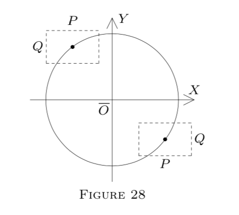
Note 4. While $H$ is unique for a given neighborhood $P \times Q$ of $(\vec{p}, \vec{q}),$ another implicit function may result if $P \times Q$ or $(\vec{p}, \vec{q})$ is changed.

For example, let

$$f(x, y)=x^{2}+y^{2}-25$$

(a polynomial; hence $f \in C D^{1}$ on all of $E^{2}).$ Geometrically, $x^{2}+y^{2}-25=0$ describes a circle.

Solving for $x,$ we get $x=\pm \sqrt{25-y^{2}}.$ Thus we have two functions:

$$H_{1}(y)=+\sqrt{25-y^{2}}$$

and

$$H_{2}(y)=-\sqrt{25-y^{2}}.$$

If $P \times Q$ is in the upper part of the circle, the resulting function is $H_{1}.$ Otherwise, it is $H_{2}.$ See Figure 28.

V. Implicit Differentiation. Theorem 4 only states the existence (and uniqueness) of a solution, but does not show how to find it, in general.

The knowledge itself that $H \in C D^{1}$ exists, however, enables us to use its derivative or partials and compute it by implicit differentiation, known from calculus.

Examples

(a) Let $f(x, y)=x^{2}+y^{2}-25=0,$ as above.

This time treating $y$ as an implicit function of $x, y=H(x),$ and writing $y^{\prime}$ for $H^{\prime}(x),$ we differentiate both sides of (x^{2}+y^{2}-25=0\) with respect to $x,$ using the chain rule for the term $y^{2}=[H(x)]^{2}$.

This yields $2 x+2 y y^{\prime}=0,$ whence $y^{\prime}=-x / y$.

Actually (see Note 4), two functions are involved: $y=\pm \sqrt{25-x^{2}};$ but both satisfy $x^{2}+y^{2}-25=0;$ so the result $y^{\prime}=-x / y$ applies to both.

Of course, this method is possible only if the derivative $y^{\prime}$ is known to exist. This is why Theorem 4 is important.

(b) Let

$$f(x, y, z)=x^{2}+y^{2}+z^{2}-1=0, \quad x, y, z \in E^{1}.$$

Again $f$ satisfies Theorem 4 for suitable $x, y,$ and $z$.

Setting $z=H(x, y),$ differentiate the equation $f(x, y, z)=0$ partially with respect to $x$ and $y.$ From the resulting two equations, obtain $\frac{\partial z}{\partial x}$ and $\frac{\partial z}{\partial y}$.