2.5: Autonomous Differential Equations
- Page ID
- 377
\( \newcommand{\vecs}[1]{\overset { \scriptstyle \rightharpoonup} {\mathbf{#1}} } \)
\( \newcommand{\vecd}[1]{\overset{-\!-\!\rightharpoonup}{\vphantom{a}\smash {#1}}} \)
\( \newcommand{\dsum}{\displaystyle\sum\limits} \)
\( \newcommand{\dint}{\displaystyle\int\limits} \)
\( \newcommand{\dlim}{\displaystyle\lim\limits} \)
\( \newcommand{\id}{\mathrm{id}}\) \( \newcommand{\Span}{\mathrm{span}}\)
( \newcommand{\kernel}{\mathrm{null}\,}\) \( \newcommand{\range}{\mathrm{range}\,}\)
\( \newcommand{\RealPart}{\mathrm{Re}}\) \( \newcommand{\ImaginaryPart}{\mathrm{Im}}\)
\( \newcommand{\Argument}{\mathrm{Arg}}\) \( \newcommand{\norm}[1]{\| #1 \|}\)
\( \newcommand{\inner}[2]{\langle #1, #2 \rangle}\)
\( \newcommand{\Span}{\mathrm{span}}\)
\( \newcommand{\id}{\mathrm{id}}\)
\( \newcommand{\Span}{\mathrm{span}}\)
\( \newcommand{\kernel}{\mathrm{null}\,}\)
\( \newcommand{\range}{\mathrm{range}\,}\)
\( \newcommand{\RealPart}{\mathrm{Re}}\)
\( \newcommand{\ImaginaryPart}{\mathrm{Im}}\)
\( \newcommand{\Argument}{\mathrm{Arg}}\)
\( \newcommand{\norm}[1]{\| #1 \|}\)
\( \newcommand{\inner}[2]{\langle #1, #2 \rangle}\)
\( \newcommand{\Span}{\mathrm{span}}\) \( \newcommand{\AA}{\unicode[.8,0]{x212B}}\)
\( \newcommand{\vectorA}[1]{\vec{#1}} % arrow\)
\( \newcommand{\vectorAt}[1]{\vec{\text{#1}}} % arrow\)
\( \newcommand{\vectorB}[1]{\overset { \scriptstyle \rightharpoonup} {\mathbf{#1}} } \)
\( \newcommand{\vectorC}[1]{\textbf{#1}} \)
\( \newcommand{\vectorD}[1]{\overrightarrow{#1}} \)
\( \newcommand{\vectorDt}[1]{\overrightarrow{\text{#1}}} \)
\( \newcommand{\vectE}[1]{\overset{-\!-\!\rightharpoonup}{\vphantom{a}\smash{\mathbf {#1}}}} \)
\( \newcommand{\vecs}[1]{\overset { \scriptstyle \rightharpoonup} {\mathbf{#1}} } \)
\(\newcommand{\longvect}{\overrightarrow}\)
\( \newcommand{\vecd}[1]{\overset{-\!-\!\rightharpoonup}{\vphantom{a}\smash {#1}}} \)
\(\newcommand{\avec}{\mathbf a}\) \(\newcommand{\bvec}{\mathbf b}\) \(\newcommand{\cvec}{\mathbf c}\) \(\newcommand{\dvec}{\mathbf d}\) \(\newcommand{\dtil}{\widetilde{\mathbf d}}\) \(\newcommand{\evec}{\mathbf e}\) \(\newcommand{\fvec}{\mathbf f}\) \(\newcommand{\nvec}{\mathbf n}\) \(\newcommand{\pvec}{\mathbf p}\) \(\newcommand{\qvec}{\mathbf q}\) \(\newcommand{\svec}{\mathbf s}\) \(\newcommand{\tvec}{\mathbf t}\) \(\newcommand{\uvec}{\mathbf u}\) \(\newcommand{\vvec}{\mathbf v}\) \(\newcommand{\wvec}{\mathbf w}\) \(\newcommand{\xvec}{\mathbf x}\) \(\newcommand{\yvec}{\mathbf y}\) \(\newcommand{\zvec}{\mathbf z}\) \(\newcommand{\rvec}{\mathbf r}\) \(\newcommand{\mvec}{\mathbf m}\) \(\newcommand{\zerovec}{\mathbf 0}\) \(\newcommand{\onevec}{\mathbf 1}\) \(\newcommand{\real}{\mathbb R}\) \(\newcommand{\twovec}[2]{\left[\begin{array}{r}#1 \\ #2 \end{array}\right]}\) \(\newcommand{\ctwovec}[2]{\left[\begin{array}{c}#1 \\ #2 \end{array}\right]}\) \(\newcommand{\threevec}[3]{\left[\begin{array}{r}#1 \\ #2 \\ #3 \end{array}\right]}\) \(\newcommand{\cthreevec}[3]{\left[\begin{array}{c}#1 \\ #2 \\ #3 \end{array}\right]}\) \(\newcommand{\fourvec}[4]{\left[\begin{array}{r}#1 \\ #2 \\ #3 \\ #4 \end{array}\right]}\) \(\newcommand{\cfourvec}[4]{\left[\begin{array}{c}#1 \\ #2 \\ #3 \\ #4 \end{array}\right]}\) \(\newcommand{\fivevec}[5]{\left[\begin{array}{r}#1 \\ #2 \\ #3 \\ #4 \\ #5 \\ \end{array}\right]}\) \(\newcommand{\cfivevec}[5]{\left[\begin{array}{c}#1 \\ #2 \\ #3 \\ #4 \\ #5 \\ \end{array}\right]}\) \(\newcommand{\mattwo}[4]{\left[\begin{array}{rr}#1 \amp #2 \\ #3 \amp #4 \\ \end{array}\right]}\) \(\newcommand{\laspan}[1]{\text{Span}\{#1\}}\) \(\newcommand{\bcal}{\cal B}\) \(\newcommand{\ccal}{\cal C}\) \(\newcommand{\scal}{\cal S}\) \(\newcommand{\wcal}{\cal W}\) \(\newcommand{\ecal}{\cal E}\) \(\newcommand{\coords}[2]{\left\{#1\right\}_{#2}}\) \(\newcommand{\gray}[1]{\color{gray}{#1}}\) \(\newcommand{\lgray}[1]{\color{lightgray}{#1}}\) \(\newcommand{\rank}{\operatorname{rank}}\) \(\newcommand{\row}{\text{Row}}\) \(\newcommand{\col}{\text{Col}}\) \(\renewcommand{\row}{\text{Row}}\) \(\newcommand{\nul}{\text{Nul}}\) \(\newcommand{\var}{\text{Var}}\) \(\newcommand{\corr}{\text{corr}}\) \(\newcommand{\len}[1]{\left|#1\right|}\) \(\newcommand{\bbar}{\overline{\bvec}}\) \(\newcommand{\bhat}{\widehat{\bvec}}\) \(\newcommand{\bperp}{\bvec^\perp}\) \(\newcommand{\xhat}{\widehat{\xvec}}\) \(\newcommand{\vhat}{\widehat{\vvec}}\) \(\newcommand{\uhat}{\widehat{\uvec}}\) \(\newcommand{\what}{\widehat{\wvec}}\) \(\newcommand{\Sighat}{\widehat{\Sigma}}\) \(\newcommand{\lt}{<}\) \(\newcommand{\gt}{>}\) \(\newcommand{\amp}{&}\) \(\definecolor{fillinmathshade}{gray}{0.9}\)A differential equation is called autonomous if it can be written as
\[ \dfrac{dy}{dt} = f(y). \nonumber \]
Notice that an autonomous differential equation is separable and that a solution can be found by integrating
\[ \int \dfrac{dy}{f(y)} = t + C \nonumber \]
Since this integral is often difficult or impossible to solve, we will investigate the solution by looking at the direction field. Direction fields of autonomous differential equations are easy to construct, since the direction field is constant for any horizontal line. One of the simplest autonomous differential equations is the one that models exponential growth.
\[ \dfrac{dy}{dt} = ry \nonumber \]
As we have seen in many prior math courses, the solution is
\[ y = C_oe^{rt}. \nonumber \]
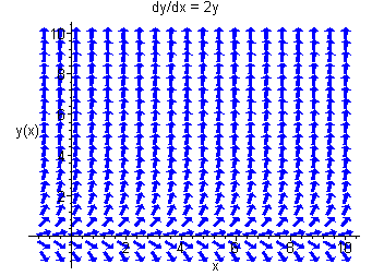
Instead of focusing on the solution, we will look at the direction field. For positive r, y' is positive for positive \(y\) and for negative \(r\), \(y'\) is negative for positive \(y\). This models exponential growth and decay as we should expect.
Below is the direction field for \(r = 2\).
The exponential model has the shortcomings of assuming that the population can increase without bound. Usually there is a limit to the population bases on space, food, and other resources. To handle this, we include a factor that will equal zero when this limit is hit. If the limit is \(K\), then the adjusted model becomes
\[ \dfrac{dy}{dt} = ry \left(1-\frac{y}{K} \right). \nonumber \]
The graph of
\[ f(y) = 2y(1-\frac{y}{50}) \nonumber \]
is shown below.
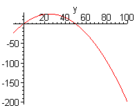
This tells us how to sketch the direction field. Sketch the direction field first for points on the y-axis. The slope is zero for \(y = 0\) and \(y = 50\), positive for \(y\) between \(0\) and \(50\) and negative elsewhere. Then repeat these slopes as we move horizontally. The direction field is shown below.
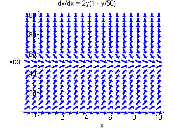
We can see that no matter what the initial population, the limiting population is 50. We call \(y = 50\) a stable equilibrium.
In nature there is another phenomenon that directs population growth. For some species, if there is not a critical mass of the species in the location, the species will become extinct. Reasons for this include the ability to find a mate and the necessity to live in a pack. This critical mass is called the threshold level. If \(T\) is the threshold level the the differential equation that models exponential growth with a threshold level is
\[ \dfrac{dy}{dt} = -ry(1-\frac{y}{T}) . \nonumber \]
Notice the similarity between the differential equations that model logistics growth and growth with a threshold. The graph of
\[ f(y) = -5y(1-\frac{y}{15}) \nonumber \]
is shown below.
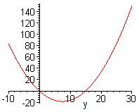
The slope is zero for \(y = 0\) and \(y = 15\), negative for y between 0 and 15 and positive elsewhere. The direction field is shown below.
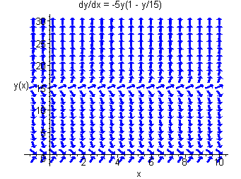
We see that if the population begins above 15, the population will increase without bound and if the population begins below 15, the species will become extinct. We call \(y = 15\) a unstable equilibrium.
If we combine the two models, we get a model for a population with both a carrying capacity and a threshold. In general the equation is
\[ \dfrac{dy}{dt} = -ry \left(1-\frac{y}{T}\right)(1-yK). \nonumber \]
The graph of
\[ f(y) = -2y(1-\frac{y}{15})(1-\frac{y}{50}) \nonumber \]
is shown below.
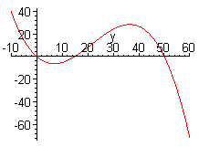
The slope is zero for \(y = 0\), \(y = 15\), and \(y = 50\), negative for y between 0 and 15 and for y greater than 50 and positive elsewhere. The direction field is shown below.
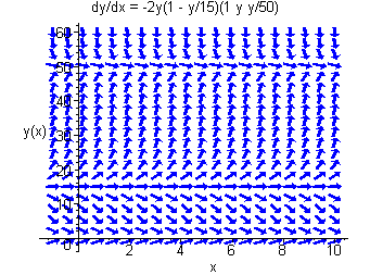
Finally consider the autonomous differential equation
\[ f(y) = y(1-\frac{y}{15})^2 . \nonumber \]
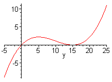
Now the slope is 0 at \(y = 0\) and \(y = 15\), but is positive for positive values of \(y\). The direction field is shown below.
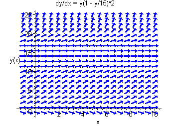
Now the line \(y = 15\) has the property that if the population starts below 15, the limiting population will tend toward 15, while if the population starts above 15 it will go away from 15. We call \(y = 15\) a semi-stable equilibrium.


