
6.8: Step Functions
- Page ID
- 395

\( \newcommand{\vecs}[1]{\overset { \scriptstyle \rightharpoonup} {\mathbf{#1}} } \)
\( \newcommand{\vecd}[1]{\overset{-\!-\!\rightharpoonup}{\vphantom{a}\smash {#1}}} \)
\( \newcommand{\dsum}{\displaystyle\sum\limits} \)
\( \newcommand{\dint}{\displaystyle\int\limits} \)
\( \newcommand{\dlim}{\displaystyle\lim\limits} \)
\( \newcommand{\id}{\mathrm{id}}\) \( \newcommand{\Span}{\mathrm{span}}\)
( \newcommand{\kernel}{\mathrm{null}\,}\) \( \newcommand{\range}{\mathrm{range}\,}\)
\( \newcommand{\RealPart}{\mathrm{Re}}\) \( \newcommand{\ImaginaryPart}{\mathrm{Im}}\)
\( \newcommand{\Argument}{\mathrm{Arg}}\) \( \newcommand{\norm}[1]{\| #1 \|}\)
\( \newcommand{\inner}[2]{\langle #1, #2 \rangle}\)
\( \newcommand{\Span}{\mathrm{span}}\)
\( \newcommand{\id}{\mathrm{id}}\)
\( \newcommand{\Span}{\mathrm{span}}\)
\( \newcommand{\kernel}{\mathrm{null}\,}\)
\( \newcommand{\range}{\mathrm{range}\,}\)
\( \newcommand{\RealPart}{\mathrm{Re}}\)
\( \newcommand{\ImaginaryPart}{\mathrm{Im}}\)
\( \newcommand{\Argument}{\mathrm{Arg}}\)
\( \newcommand{\norm}[1]{\| #1 \|}\)
\( \newcommand{\inner}[2]{\langle #1, #2 \rangle}\)
\( \newcommand{\Span}{\mathrm{span}}\) \( \newcommand{\AA}{\unicode[.8,0]{x212B}}\)
\( \newcommand{\vectorA}[1]{\vec{#1}} % arrow\)
\( \newcommand{\vectorAt}[1]{\vec{\text{#1}}} % arrow\)
\( \newcommand{\vectorB}[1]{\overset { \scriptstyle \rightharpoonup} {\mathbf{#1}} } \)
\( \newcommand{\vectorC}[1]{\textbf{#1}} \)
\( \newcommand{\vectorD}[1]{\overrightarrow{#1}} \)
\( \newcommand{\vectorDt}[1]{\overrightarrow{\text{#1}}} \)
\( \newcommand{\vectE}[1]{\overset{-\!-\!\rightharpoonup}{\vphantom{a}\smash{\mathbf {#1}}}} \)
\( \newcommand{\vecs}[1]{\overset { \scriptstyle \rightharpoonup} {\mathbf{#1}} } \)
\(\newcommand{\longvect}{\overrightarrow}\)
\( \newcommand{\vecd}[1]{\overset{-\!-\!\rightharpoonup}{\vphantom{a}\smash {#1}}} \)
\(\newcommand{\avec}{\mathbf a}\) \(\newcommand{\bvec}{\mathbf b}\) \(\newcommand{\cvec}{\mathbf c}\) \(\newcommand{\dvec}{\mathbf d}\) \(\newcommand{\dtil}{\widetilde{\mathbf d}}\) \(\newcommand{\evec}{\mathbf e}\) \(\newcommand{\fvec}{\mathbf f}\) \(\newcommand{\nvec}{\mathbf n}\) \(\newcommand{\pvec}{\mathbf p}\) \(\newcommand{\qvec}{\mathbf q}\) \(\newcommand{\svec}{\mathbf s}\) \(\newcommand{\tvec}{\mathbf t}\) \(\newcommand{\uvec}{\mathbf u}\) \(\newcommand{\vvec}{\mathbf v}\) \(\newcommand{\wvec}{\mathbf w}\) \(\newcommand{\xvec}{\mathbf x}\) \(\newcommand{\yvec}{\mathbf y}\) \(\newcommand{\zvec}{\mathbf z}\) \(\newcommand{\rvec}{\mathbf r}\) \(\newcommand{\mvec}{\mathbf m}\) \(\newcommand{\zerovec}{\mathbf 0}\) \(\newcommand{\onevec}{\mathbf 1}\) \(\newcommand{\real}{\mathbb R}\) \(\newcommand{\twovec}[2]{\left[\begin{array}{r}#1 \\ #2 \end{array}\right]}\) \(\newcommand{\ctwovec}[2]{\left[\begin{array}{c}#1 \\ #2 \end{array}\right]}\) \(\newcommand{\threevec}[3]{\left[\begin{array}{r}#1 \\ #2 \\ #3 \end{array}\right]}\) \(\newcommand{\cthreevec}[3]{\left[\begin{array}{c}#1 \\ #2 \\ #3 \end{array}\right]}\) \(\newcommand{\fourvec}[4]{\left[\begin{array}{r}#1 \\ #2 \\ #3 \\ #4 \end{array}\right]}\) \(\newcommand{\cfourvec}[4]{\left[\begin{array}{c}#1 \\ #2 \\ #3 \\ #4 \end{array}\right]}\) \(\newcommand{\fivevec}[5]{\left[\begin{array}{r}#1 \\ #2 \\ #3 \\ #4 \\ #5 \\ \end{array}\right]}\) \(\newcommand{\cfivevec}[5]{\left[\begin{array}{c}#1 \\ #2 \\ #3 \\ #4 \\ #5 \\ \end{array}\right]}\) \(\newcommand{\mattwo}[4]{\left[\begin{array}{rr}#1 \amp #2 \\ #3 \amp #4 \\ \end{array}\right]}\) \(\newcommand{\laspan}[1]{\text{Span}\{#1\}}\) \(\newcommand{\bcal}{\cal B}\) \(\newcommand{\ccal}{\cal C}\) \(\newcommand{\scal}{\cal S}\) \(\newcommand{\wcal}{\cal W}\) \(\newcommand{\ecal}{\cal E}\) \(\newcommand{\coords}[2]{\left\{#1\right\}_{#2}}\) \(\newcommand{\gray}[1]{\color{gray}{#1}}\) \(\newcommand{\lgray}[1]{\color{lightgray}{#1}}\) \(\newcommand{\rank}{\operatorname{rank}}\) \(\newcommand{\row}{\text{Row}}\) \(\newcommand{\col}{\text{Col}}\) \(\renewcommand{\row}{\text{Row}}\) \(\newcommand{\nul}{\text{Nul}}\) \(\newcommand{\var}{\text{Var}}\) \(\newcommand{\corr}{\text{corr}}\) \(\newcommand{\len}[1]{\left|#1\right|}\) \(\newcommand{\bbar}{\overline{\bvec}}\) \(\newcommand{\bhat}{\widehat{\bvec}}\) \(\newcommand{\bperp}{\bvec^\perp}\) \(\newcommand{\xhat}{\widehat{\xvec}}\) \(\newcommand{\vhat}{\widehat{\vvec}}\) \(\newcommand{\uhat}{\widehat{\uvec}}\) \(\newcommand{\what}{\widehat{\wvec}}\) \(\newcommand{\Sighat}{\widehat{\Sigma}}\) \(\newcommand{\lt}{<}\) \(\newcommand{\gt}{>}\) \(\newcommand{\amp}{&}\) \(\definecolor{fillinmathshade}{gray}{0.9}\)In this discussion, we will investigate piecewise defined functions and their Laplace Transforms. We start with the fundamental piecewise defined function, the Heaviside function.
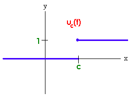
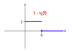
The Heaviside function, also called the unit step function, is defined by
\[ u_c(t) = \left\{\begin{aligned}
&1 && t <c \\
&0 && t \ge c
\end{aligned}
\right. \nonumber \]
for \(c \ge 0\).
The Heaviside function \(y = u_c(t)\) and \(y = 1 - u_c(t)\) are graphed below.
We can write the function
\[ f(t) = \left\{\begin{aligned}
&3 && 0 \le x < 2 \\ &e^x && 2 \le x < 5 \\ &0 && 5 \le x
\end{aligned}
\right. \nonumber \]
in terms of Heaviside functions.
Solution
We tackle the functions in parts. The function that is 1 from 0 to 2, and 0 otherwise is
\[1 - u_2(x) . \nonumber \]
Multiplying by 3 gives
\[ 3\left(1 - u_2(x)\right) = 3 - 3u_2(x) . \nonumber \]
To get the function that is 1 between 2 and 5 and 0 otherwise, we subtract
\[ u_2(x) - u_5(x) . \nonumber \]
Now multiply by \(e^x\) to get
\[ e^x(u_2(x) - u_5(x)) = e^x u_2(x) - e^x u_5(x). \nonumber \]
Adding these together gives
\[\begin{align} f(x) &= 3 - 3u_2(x) + e^x\, u_2(x) - e^x \,u_5(x) \\ &= 3 + (e^x - 3)\,u_2(x) - e^x\, u_5(x) . \end{align} \nonumber \]
We can find the Laplace transform of \(u_c(t)\) by integrating
\[ \mathcal{L}\{u_c(t)\} = \int_0^{\infty} e^{st} u_c(t) \, dt \nonumber \]
\[ = \int _c^{\infty} e^{st} dt = \dfrac{e^{-cs}}{s} \nonumber \]
\[ L \{ u_c(t)\} = \dfrac{e^{-cs}}{s}. \nonumber \]
In practice, we want to find the Laplace transform of a more general piecewise defined function such as
\[ f(t) = \left\{\begin{aligned}
&0 && x < \pi \\ &\sin x && x \ge \pi
\end{aligned}
\right. \nonumber \]
This type of function occurs in electronics when a switch is suddenly turned on after one second and a forcing function is applied. We can write
\[ f(x) = u_p(x) \sin x. \nonumber \]
We will be interested in the Laplace transform of a product of the Heaviside function with a continuous function. The result that we need is
\[ \mathcal{L}\{(u_c(t) f(t - c)\} = e^{-cs} \mathcal{L}\{f(t)\} . \nonumber \]
By taking inverses we get that if \(F(s) = \mathcal{L}\{f(t)\}\), then
\[ L^{-1}\{e^{-cs}F(s)\} = u_c(t)f(t - c) . \nonumber \]
Proof
We use the definition to get
\[ \mathcal{L}\{u_c(t)f(t-c)\} = \int _0^{\infty} e^{-st}u_c(t)f(t-c)\,dt \nonumber \]
substitute \(\nu=t-c\)
\[ = \int _c^{\infty} e^{-st}f(t-c)\,dt = \int _0^{\infty} e^{-(\nu +c)s}f(\nu)\,d\nu \nonumber \]
\[ e^{-cs}\int _0^{\infty} e^{-s\nu}f(\nu)\,d\nu = e^{-cs}F(s). \nonumber \]
Find the Laplace transform of
\[ f(t) = \left\{\begin{aligned}
&0 && x < \pi \\ &\sin x && x \ge \pi.
\end{aligned}
\right. \nonumber \]
Solution
We use that fact that
\[ f(x) = u_p(x) \sin x = -u_p(x) \sin[(x - p)] . \nonumber \]
Now we can use the formula to get that
\[ \mathcal{L}\{f(x)\} = -\mathcal{L}\{u_p(x) \sin[(x - p)]\} = -e^{-cs} \mathcal{L}\{\sin x\}. \nonumber \]
By the table of Laplace Transforms, we get
\[ = \dfrac{-e^{-cs}}{s^2 + 1} . \nonumber \]