
1.1: Onto Several Variables
- Page ID
- 74222

Let \(\mathbb{C}^n = \overbrace{\mathbb{C} \times \mathbb{C} \times \cdots \times \mathbb{C}}^{\text{$n$ times}}\) denote the \(n\)-dimensional complex Euclidean space. Denote by \(z = (z_1,z_2,\ldots,z_n)\) the coordinates of \(\mathbb{C}^n\). Let \(x = (x_1,x_2,\ldots,x_n)\) and \(y = (y_1,y_2,\ldots,y_n)\) denote coordinates in \(\mathbb{R}^n\). We identify \(\mathbb{C}^n\) with \(\mathbb{R}^{2n}\) by letting \(z = x+iy\), that is, \(z_j = x_j + i y_j\) for every \(j\). As in one complex variable, we write \(\bar{z} = x-iy\). We call \(z\) the holomorphic coordinates and \(\bar{z}\) the antiholomorphic coordinates.
For \(\rho = (\rho_1,\rho_2,\ldots,\rho_n)\) where \(\rho_j > 0\) and \(a \in \mathbb{C}^n\), define a polydisc \[\Delta_\rho(a) \overset{\text{def}}{=} \bigl\{ z \in \mathbb{C}^n : |z_j - a_j| < \rho_j ~\text{for $j=1,2,\ldots,n$} \bigr\} .\]
Call \(a\) the center and \(\rho\) the polyradius or simply the radius of the polydisc \(\Delta_\rho(a)\). If \(\rho > 0\) is a number, then \[\Delta_\rho(a) \overset{\text{def}}{=} \bigl\{ z \in \mathbb{C}^n : |z_j - a_j| < \rho ~\text{for $j=1,2,\ldots,n$} \bigr\} .\] In two variables, a polydisc is sometimes called a bidisc.
As there is the unit disc \(\mathbb{D}\) in one variable, so is there the unit polydisc in several variables: \[\mathbb{D}^n = \mathbb{D} \times \mathbb{D} \times \cdots \times \mathbb{D} = \Delta_1(0) = \bigl\{ z \in \mathbb{C}^n : |z_j| < 1 ~\text{for $j=1,2,\ldots,n$} \bigr\} .\]
In more than one complex dimension, it is difficult to draw exact pictures for lack of real dimensions on our paper. We visualize the unit polydisc in two variables (bidisc) as in by plotting against the modulus of the variables.
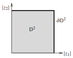
Figure \(\PageIndex{1}\)
Recall the Euclidean inner product on \(\mathbb{C}^n\): \[\langle z,w\rangle \overset{\text{def}}{=} z \cdot \bar{w} z_1 \bar{w}_1 + z_2 \bar{w}_2 + \cdots + z_n \bar{w}_n .\] The inner product gives us the standard Euclidean norm on \(\mathbb{C}^n\): \[||z|| \overset{\text{def}}{=} \sqrt{\langle z,z\rangle } = \sqrt{|z_1|^2 + |z_2|^2 + \cdots + |z_n|^2} .\] This norm agrees with the standard Euclidean norm on \(\mathbb{R}^{2n}\). Define balls as in \(\mathbb{R}^{2n}\): \[B_\rho(a) \overset{\text{def}}{=} \bigl\{ z \in \mathbb{C}^n : ||z - a|| < \rho \bigr\} ,\] And the unit ball, \[\mathbb{B}_{n} \overset{\text{def}}{=} B_1(0) = \bigl\{ z \in \mathbb{C}^n : ||z|| < 1 \bigr\} .\]
A ball centered at the origin can also be pictured by plotting against the modulus of the variables since the inequality defining the ball only depends on the moduli of the variables. Not every domain can be drawn like this, but if it can, it is called a Reinhardt domain, more on this later. A picture of \(\mathbb{B}_{2}\) is in Figure \(\PageIndex{2}\).
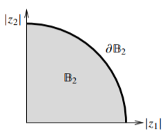
Figure \(\PageIndex{2}\)
Let \(U \subset \mathbb{C}^n\) be open. A function \(f \colon U \to \mathbb{C}\) is holomorphic if it is locally bounded\(^{1}\) and holomorphic in each variable separately. That is, \(f\) is holomorphic if it is locally bounded and complex-differentiable in each variable separately: \[\lim_{\xi \in \mathbb{C}\to 0} \frac{f(z_1,\ldots,z_k+\xi,\ldots,z_n) - f(z)}{\xi} \qquad \text{exists for all $z \in U$ and all $k=1,2,\ldots,n$}.\] In this book, however, the words “differentiable” and “derivative” (without the “complex-”) refer to plain vanilla real differentiability.
As in one variable, we define the Wirtinger operators \[\frac{\partial}{\partial z_k} \overset{\text{def}}{=} \frac{1}{2} \left( \frac{\partial}{\partial x_k} - i \frac{\partial}{\partial y_k} \right) , \qquad \frac{\partial}{\partial \bar{z}_k} \overset{\text{def}}{=} \frac{1}{2} \left( \frac{\partial}{\partial x_k} + i \frac{\partial}{\partial y_k} \right) .\] An alternative definition is to say that a continuously differentiable function \(f \colon U \to \mathbb{C}\) is holomorphic if it satisfies the Cauchy-Riemann equations \[\frac{\partial f}{\partial \bar{z}_k} = 0 \qquad \text{for $k=1,2,\ldots,n$}.\] For holomorphic functions, using the natural definition for partial derivatives obtains the the Wirtinger \(\frac{\partial}{\partial z_k}\). Namely, if \(f\) is holomorphic, then \[\frac{\partial f}{\partial z_k}(z) = \lim_{\xi \in \mathbb{C} \to 0} \frac{f(z_1,\ldots,z_k+\xi,\ldots,z_n) - f(z)}{\xi} .\]
Due to the following proposition, the alternative definition using the Cauchy–Riemann equations is just as good as the definition we gave. In the proof, if you wish to stay with just the Riemann integral instead of the Lebesgue integral, feel free to assume that \(f\) is continuously differentiable.
Let \(U \subset \mathbb{C}^n\) be an open set and suppose \(f \colon U \to \mathbb{C}\) is holomorphic. Then \(f\) is infinitely differentiable.
- Proof
-
Suppose \(\Delta = \Delta_{\rho}(a) = \Delta_1 \times \cdots \times \Delta_n\) is a polydisc centered at \(a\), where each \(\Delta_j\) is a disc and suppose \(\overline{\Delta} \subset U\), that is, \(f\) is holomorphic on a neighborhood of the closure of \(\Delta\). Let \(z\) be in \(\Delta\). Orient \(\partial \Delta_1\) positively and apply the Cauchy formula (after all \(f\) is holomorphic in \(z_1\)): \[f(z) = \frac{1}{2\pi i} \int_{\partial \Delta_1} \frac{f(\zeta_1,z_2,\ldots,z_n)}{\zeta_1-z_1} \, d \zeta_1 .\] Apply it again on the second variable, again orienting \(\partial \Delta_2\) positively: \[f(z) = \frac{1}{{(2\pi i)}^2} \int_{\partial \Delta_1} \int_{\partial \Delta_2} \frac{f(\zeta_1,\zeta_2,z_3,\ldots,z_n)}{(\zeta_1-z_1)(\zeta_2-z_2)} \, d \zeta_2 \, d \zeta_1 .\]
Applying the formula \(n\) times we obtain \[\label{eq:1} f(z) = \frac{1}{{(2\pi i)}^n} \int_{\partial \Delta_1} \int_{\partial \Delta_2} \cdots \int_{\partial \Delta_n} \frac{f(\zeta_1,\zeta_2,\ldots,\zeta_n)}{(\zeta_1-z_1)(\zeta_2-z_2)\cdots(\zeta_n-z_n)} \, d \zeta_n \cdots d \zeta_2 \, d \zeta_1 .\] As \(f\) is bounded on the compact set \(\partial \Delta_1 \times \cdots \times \partial \Delta_n\), we find that \(f\) is continuous in \(\Delta\). We may differentiate underneath the integral, because \(f\) is bounded on \(\partial \Delta_1 \times \cdots \times \partial \Delta_n\) and so are the derivatives of the integrand with respect to \(x_j\) and \(y_j\), where \(z_j=x_j+i y_j\), as long as \(z\) is a positive distance away from \(\partial \Delta_1 \times \cdots \times \partial \Delta_n\). We may differentiate as many times as we wish.
In \(\eqref{eq:1}\) above, we derived the Cauchy integral formula in several variables. To write the formula more concisely we apply the Fubini’s theorem to write it as a single integral. We will write it down using differential forms. If you are unfamiliar with differential forms, think of the integral as the iterated integral above, and you can read the next few paragraphs a little lightly. It is enough to understand real differential forms; we simply allow complex coefficients here. See Appendix C for an overview of differential forms, or Rudin [R2] for an introduction with all the details.
Given real coordinates \(x = (x_1,\ldots,x_n)\), a one-form \(d x_k\) is a linear functional on tangent vectors such that \(d x_k \bigl( \frac{\partial}{\partial x_k} \bigr) = 1\) and \(d x_k \bigl( \frac{\partial}{\partial x_{\ell}} \bigr) = 0\) if \(k \not= {\ell}\). Because \(z_k = x_k + i y_k\) and \(\bar{z}_k = x_k - i y_k\), \[d z_k = d x_k + i \, d y_k , \qquad d \bar{z}_k = d x_k - i \, d y_k .\] Let \(\delta_{k}^{\ell}\) be the Kronecker delta, that is, \(\delta_k^k = 1\), and \(\delta_k^{\ell} = 0\) if \(k \not= {\ell}\). Then as expected, \[d z_k \left( \frac{\partial}{\partial z_{\ell}} \right) = \delta_k^{\ell} , \qquad d z_k \left( \frac{\partial}{\partial \bar{z}_{\ell}} \right) = 0 , \qquad d \bar{z}_k \left( \frac{\partial}{\partial z_{\ell}} \right) = 0 , \qquad d \bar{z}_k \left( \frac{\partial}{\partial \bar{z}_{\ell}} \right) = \delta_k^{\ell} .\] One-forms are objects of the form \[\sum_{k=1}^n \alpha_k \, d z_k + \beta_k \, d \bar{z}_k ,\] where \(\alpha_k\) and \(\beta_k\) are functions (of \(z\)). Two-forms are combinations of wedge products, \(\omega \wedge \eta\), of one-forms. A wedge of a two-form and a one-form is a three-form, etc. An \(m\)-form is an object that can be integrated on a so-called \(m\)-chain, for example, a \(m\)-dimensional surface. The wedge product takes care of the orientation as it is anticommutative on one-forms: For one-forms \(\omega\) and \(\eta\), we have \(\omega \wedge \eta = - \eta \wedge \omega\).
At this point, we need to talk about orientation in \(\mathbb{C}^n\), that is, ordering of the real coordinates. There are two natural real-linear isomorphisms of \(\mathbb{C}^n\) and \(\mathbb{R}^{2n}\). We identify \(z = x+iy\) as either \[(x,y) = (x_1,\ldots,x_n,y_1,\ldots,y_n) \qquad \text{or} \qquad (x_1,y_1,x_2,y_2,\ldots,x_n,y_n) .\] If we take the natural orientation of \(\mathbb{R}^{2n}\), it is possible (if \(n\) is even) that we obtain two opposite orientations on \(\mathbb{C}^n\) (if \(n\) is even, the real linear map that takes one ordering to the other has determinant \(-1\)). The orientation we take as the natural orientation of \(\mathbb{C}^n\) (in this book) corresponds to the second ordering above, that is, \((x_1,y_1,\ldots,x_n,y_n)\). Either isomorphism may be used in computation as long as it is used consistently, and the underlying orientation is kept in mind.
Cauchy Integral Formula
Let \(\Delta \subset \mathbb{C}^n\) be a polydisc. Suppose \(f \colon \overline{\Delta} \to \mathbb{C}\) is a continuous function holomorphic in \(\Delta\). Write \(\Gamma = \partial \Delta_1 \times \cdots \times \partial \Delta_n\) oriented appropriately (each \(\partial \Delta_j\) has positive orientation). Then for \(z \in \Delta\) \[f(z) = \frac{1}{{(2\pi i)}^n} \int_{\Gamma} \frac{f(\zeta_1,\zeta_2,\ldots,\zeta_n)}{(\zeta_1-z_1)(\zeta_2-z_2)\cdots(\zeta_n-z_n)} \, d \zeta_1 \wedge d \zeta_2 \wedge \cdots \wedge d \zeta_n .\]
We stated a more general result where \(f\) is only continuous on \(\overline{\Delta}\) and holomorphic in \(\Delta\). The proof of this slight generalization is contained within the next two exercises.
Suppose \(f \colon \overline{\mathbb{D}^2} \to \mathbb{C}\) is continuous and holomorphic on \(\mathbb{D}^2\). For every \(\theta \in \mathbb{R}\), prove \[g_1(\xi) = f(\xi,e^{i\theta}) \qquad \text{and} \qquad g_2(\xi) = f(e^{i\theta},\xi) \] are holomorphic in \(\mathbb{D}\).
Prove the theorem above, that is, the slightly more general Cauchy integral formula where \(f\) is only continuous on \(\overline{\Delta}\) and holomorphic in \(\Delta\).
The Cauchy integral formula shows an important and subtle point about holomorphic functions in several variables: The value of the function \(f\) on \(\Delta\) is completely determined by the values of \(f\) on the set \(\Gamma\), which is much smaller than the boundary of the polydisc \(\partial \Delta\). In fact, the \(\Gamma\) is of real dimension \(n\), while the boundary of the polydisc has real dimension \(2n-1\). The set \(\Gamma = \partial \Delta_1 \times \cdots \times \partial \Delta_n\) is called the distinguished boundary. See for the distinguished boundary of the bidisc.
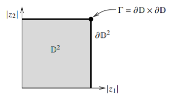
Figure \(\PageIndex{3}\)
The set \(\Gamma\) is a 2-dimensional torus, like the surface of a donut. Whereas the set \(\partial \mathbb{D}^2 = (\partial \mathbb{D} \times \overline{\mathbb{D}}) \cup (\overline{\mathbb{D}} \times \partial \mathbb{D})\) is the union of two filled donuts, or more precisely it is both the inside and the outside of the donut put together, and these two things meet on the surface of the donut. So the set \(\Gamma\) is quite small in comparison to the entire boundary \(\partial \mathbb{D}^2\).
Suppose \(\Delta\) is a polydisc, \(\Gamma\) its distinguished boundary, and \(f \colon \overline{\Delta} \to \mathbb{C}\) is continuous on \(\overline{\Delta}\) and holomorphic on \(\Delta\). Prove \(|f(z)|\) achieves its maximum on \(\Gamma\).
A ball and is different from a polydisc. Prove that for every \(p \in \partial \mathbb{B}_{n}\) there exists a continuous \(f \colon \overline{\mathbb{B}_{n}} \to \mathbb{C}\), holomorphic on \(\mathbb{B}_{n}\), such that \(|f(z)|\) achieves a strict maximum at \(p\).
Show that in the real setting, differentiable in each variable separately does not imply differentiable even if the function is locally bounded. Let \(f(x,y) = \frac{xy}{x^2+y^2}\) outside the origin and \(f(0,0) = 0\). Prove that \(f\) is a locally bounded function in \(\mathbb{R}^2\), which is differentiable in each variable separately (all partial derivatives exist at every point), but \(f\) is not even continuous. There is something very special about the holomorphic category.
Suppose \(U \subset \mathbb{C}^n\) is open. Prove that \(f \colon U \to \mathbb{C}\) is holomorphic if and only if \(f\) is locally bounded and for every \(a,b \in \mathbb{C}^n\), the function \(\zeta \mapsto f(\zeta a + b)\) is holomorphic on the open set \(\{ \zeta \in \mathbb{C} : \zeta a + b \in U \}\).
Prove a several complex variables version of Morera’s theorem (see Theorem B.4). A triangle \(T \subset \mathbb{C}^n\) is the closed convex hull of three points, so including the inside. Orient \(T\) in some way and orient \(\partial T\) accordingly. A triangle \(T\) lies in a complex line if its vertices \(a,b,c\) satisfy \(\zeta (b-a) = c-a\) for some \(\zeta \in \mathbb{C}\). Suppose \(U \subset \mathbb{C}^n\) is open and \(f \colon U \to \mathbb{C}\) is continuous. Prove that \(f\) is holomorphic if and only if \[\int_{\partial T} f(z) \, dz_k = 0\] for every triangle \(T \subset U\) that lies in a complex line, and every \(k=1,2,\ldots,n\). Hint: The previous exercise may be useful.
For \(0 < \epsilon < 1\), suppose a continuous \(f \colon \overline{\mathbb{D}^2} \setminus \overline{\Delta_\epsilon(0)} \to \mathbb{C}\) is holomorphic on \(\mathbb{D}^2 \setminus \overline{\Delta_\epsilon(0)}\). Prove that \(f\) is bounded.
Footnotes
[1] For every \(p \in U\), there is a neighborhood \(N\) of \(p\) such that \(f|_N\) is bounded. It is a deep result of Hartogs that we might in fact just drop “locally bounded” from the definition and obtain the same set of functions.