
1.2: Power Series Representation


- Last updated
- Sep 5, 2021
- Save as PDF

( \newcommand{\kernel}{\mathrm{null}\,}\)
As you noticed, writing out all the components can be a pain. Just as we write vectors as z instead of (z1,z2,…,zn), we similarly define the so-called multi-index notation to deal with more complicated formulas such as the ones above.
Let α∈Nn0 be a vector of nonnegative integers (where N0=N∪{0}). We write zαdef=zα11zα22⋯zαnn,|z|αdef=|z1|α1|z2|α2⋯|zn|αn,1zdef=1z1z2⋯zn,zwdef=(z1w1,z2w2,…,znwn),∂|α|∂zαdef=∂α1∂zα11∂α2∂zα22⋯∂αn∂zαnn,dzdef=dz1∧dz2∧⋯∧dzn,|α|def=α1+α2+⋯+αn,α!def=α1!α2!⋯αn!. We can also make sense of this notation, especially the notation zα, if α∈Zn, that is, if it includes negative integers. Although usually, α is assumed to be in Nn0. Furthermore, when we use 1 as a vector it means (1,1,…,1). If z∈Cn, then 1−z=(1−z1,1−z2,…,1−zn),orzα+1=zα1+11zα2+12⋯zαn+1n. It goes without saying that when using this notation it is important to be careful to always realize which symbol lives where, and most of all, to not get carried away. For instance, one could interpret 1z in two different ways depending on if we interpret 1 as a vector or not, and if we are expecting a vector or a number. Best to just keep to the limited set of cases as given above.
In this notation, the Cauchy formula becomes the perhaps deceptively simple f(z)=1(2πi)n∫Γf(ζ)ζ−zdζ.
Let us move to power series. For simplicity, we start with power series at the origin. Using the multinomial notation, we write such a series as ∑α∈Nn0cαzα. You must admit that the above is far nicer to write than writing, for example, in C3, ∞∑j=0∞∑k=0∞∑ℓ=0cjkℓzj1zk2zℓ3, which is not even exactly the definition of the series sum (see below). When it is clear from context that we are talking about a power series and all the powers are nonnegative, we write simply ∑αcαzα.
It is important to note what this means. The sum does not have a natural ordering. We are summing over α∈Nn0, and there is no natural ordering of Nn0. It makes no sense to talk about conditional convergence. When we say the series converges , we mean absolutely. Fortunately, power series converge absolutely, and so the ordering does not matter. If you want to write the limit in terms of partial sums, you pick some ordering of the multi-indices, α(1),α(2),…, and then ∑αcαzα=limm→∞m∑k=1cα(k)zα(k). By the Fubini theorem (for sums) this limit is equal to the iterated sum such as (???).
A power series ∑αcαzα converges uniformly absolutely for z∈X when ∑α|cαzα| converges uniformly for z∈X. The geometric series in several variables is the series ∑αzα. For z∈Dn (unit polydisc), 11−z=1(1−z1)(1−z2)⋯(1−zn)=(∞∑k=0z1k)(∞∑k=0z2k)⋯(∞∑k=0znk)=∞∑k1=0∞∑k2=0⋯∞∑kn=0(z1k1znk2⋯znkn)=∑αzα. The series converges uniformly absolutely on all compact subsets of the unit polydisc: Any compact set in the unit polydisc is contained in a closed polydisc ¯Δ centered at 0 of radius 1−ϵ for some ϵ>0. The convergence is uniformly absolute on ¯Δ. This claim follows by simply noting the same fact for each factor is true in one dimension.
Holomorphic functions are precisely those having a power series expansion:
Let Δ=Δρ(a)⊂Cn be a polydisc. Suppose f:¯Δ→C is a continuous function holomorphic in Δ. Then on Δ, f is equal to a power series converging uniformly absolutely on compact subsets of Δ: f(z)=∑αcα(z−a)α.
Conversely, if f:Δ→C is defined by (???) converging uniformly absolutely on compact subsets of Δ, then f is holomorphic on Δ.
- Proof
-
Suppose a continuous f:¯Δ→C is holomorphic on Δ. Let Γ=∂Δ1×⋯×∂Δn be oriented positively. Take z∈Δ and ζ∈Γ. As in one variable, write the Cauchy kernel as 1ζ−z=1ζ−a1(1−z−aζ−a)=1ζ−a∑α(z−aζ−a)α. Interpret the formulas as 1ζ−z=1(ζ1−z1)⋯(ζn−zn), 1ζ−a=1(ζ1−a1)⋯(ζn−an) and z−aζ−a=(z1−a1ζ1−a1,…,zn−anζn−an).
The multivariable geometric series is a product of geometric series in one variable, and geometric series in one variable are uniformly absolutely convergent on compact subsets of the unit disc. So the series above converges uniformly absolutely for (z,ζ)∈K×Γ for every compact subset K of Δ.
Compute,
f(z)=1(2πi)n∫Γf(ζ)ζ−zdζ=1(2πi)n∫Γf(ζ)ζ−a∑α(z−aζ−a)αdζ=∑α(1(2πi)n∫Γf(ζ)(ζ−a)α+1dζ)(z−a)a.
The last equality follows by Fubini or uniform convergence just as it does in one variable.
Uniform absolute convergence (as z moves) on compact subsets of the final series follows from the uniform absolute convergence of the geometric series. It is also a direct consequence of the Cauchy estimates below.
We have shown that f(z)=∑αcα(z−a)α, where cα=1(2πi)n∫Γf(ζ)(ζ−a)α+1dζ.
Notice how strikingly similar the computation is to one variable.
Let us prove the converse statement. The limit of the series is continuous as it is a uniform-on-compact-sets limit of continuous functions, and hence it is locally bounded in Δ. Next, we restrict to each variable in turn, zj↦∑αcα(z−a)α. This function is holomorphic via the corresponding one-variable argument.
The converse statement also follows by applying the Cauchy–Riemann equations to the series termwise. We leave that as an exercise. First, one must show that the term-by-term derivative series also converges uniformly absolutely on compact subsets. Then one applies the theorem from real analysis about derivatives of limits: If a sequence of functions and its derivatives converges uniformly, then the derivatives converge to the derivative of the limit.
Prove the claim above that if a power series converges uniformly absolutely on compact subsets of a polydisc Δ, then the term-by-term derivative converges. Do the proof without using the analogous result for single variable series.
A third way to prove the converse statement of the theorem is to note that partial sums are holomorphic and write them using the Cauchy formula. Uniform convergence shows that the limit also satisfies the Cauchy formula, and differentiating under the integral obtains the result.
Follow the logic above to prove the converse of the theorem, without using the analogous result for single variable series. Hint: Let Δ″ be two polydiscs with the same center a such that \overline{\Delta''} \subset \Delta' and \overline{\Delta'} \subset \Delta. Apply Cauchy formula on \Delta' for z \in \overline{\Delta''}.
We organize some consequences of the theorem and the calculation in the proof.
Let \Delta = \Delta_\rho(a) \subset \mathbb{C}^n be a polydisc, and \Gamma its distinguished boundary. Suppose f \colon \overline{\Delta} \to \mathbb{C} is a continuous function holomorphic in \Delta. Then, for z \in \Delta,
\frac{\partial^{|\alpha |}f}{\partial z^{\alpha}}(z)=\frac{1}{(2\pi i)^{n}}\int_{\Gamma}\frac{\alpha !f(\zeta )}{(\zeta -z)^{\alpha +1}}d\zeta .
In particular, if f is given by \eqref{eq:2}, then c_\alpha = \frac{1}{\alpha!} \frac{\partial^{|\alpha|}f}{\partial z^\alpha} (a), and we have the Cauchy estimates: |c_\alpha| \leq \frac{||f||_\Gamma}{\rho^\alpha} .
Namely, the coefficients of the power series depend only on the derivatives of f at a (and so on the values of f in an arbitrarily small neighborhood of a) and not the specific polydisc used in the theorem.
- Proof
-
By the Leibniz rule (taking derivatives under the integral), if z \in \Delta (not on the boundary), we can differentiate under the integral. We are talking regular real partial differentiation, and we use it to apply the Wirtinger operator. The point is that
\frac{\partial}{\partial z_{\ell}}\left[\frac{1}{(\zeta_{\ell}-z_{\ell})^{k}}\right]=\frac{k}{(\zeta_{\ell}-z_{\ell})^{k+1}}.
Let us do a single derivative to get the idea: \begin{align}\begin{aligned} \frac{\partial f}{\partial z_1}(z) &= \frac{\partial}{\partial z_1} \left[ \frac{1}{{(2\pi i)}^n} \int_{\Gamma} \frac{f(\zeta_1,\zeta_2,\ldots,\zeta_n)}{(\zeta_1-z_1)(\zeta_2-z_2)\cdots(\zeta_n-z_n)} \, d \zeta_1 \wedge d \zeta_2 \wedge \cdots \wedge d \zeta_n \right] \\ & = \frac{1}{{(2\pi i)}^n} \int_{\Gamma} \frac{f(\zeta_1,\zeta_2,\ldots,\zeta_n)}{{(\zeta_1-z_1)}^2(\zeta_2-z_2)\cdots(\zeta_n-z_n)} \, d \zeta_1 \wedge d \zeta_2 \wedge \cdots \wedge d \zeta_n . \end{aligned}\end{align} How about we do it a second time: \frac{\partial^2 f}{\partial z_1^2}(z) = \frac{1}{{(2\pi i)}^n} \int_{\Gamma} \frac{2 f(\zeta_1,\zeta_2,\ldots,\zeta_n)}{{(\zeta_1-z_1)}^3(\zeta_2-z_2)\cdots(\zeta_n-z_n)} \, d \zeta_1 \wedge d \zeta_2 \wedge \cdots \wedge d \zeta_n . Notice the 2 before the f. Next derivative, a 3 is coming out. After j derivatives in z_1 you get the constant j!. It is exactly the same thing that happens in one variable. A moment’s thought will convince you that the following formula is correct for \alpha \in \mathbb{N}_0^n:
\frac{\partial^{|\alpha |}f}{\partial z^{\alpha}}(z)=\frac{1}{(2\pi i)^{n}}\int_{\Gamma}\frac{\alpha !f(\zeta )}{(\zeta -z)^{\alpha +1}}d\zeta .
Therefore, \alpha! \, c_\alpha = \frac{\partial^{|\alpha|} f}{\partial z^\alpha} (a) . We obtain the Cauchy estimates as before:
\left|\frac{\partial^{|\alpha |}f}{\partial z^{\alpha}}(a)\right|=\left|\frac{1}{(2\pi i)^{n}}\int_{\Gamma}\frac{\alpha ! f(\zeta)}{(\zeta -a)^{\alpha +1}}d\zeta \right|\leq\frac{1}{(2\pi )^{n}}\int_{\Gamma}\frac{\alpha !|f(\zeta )|}{\rho^{\alpha +1}}|d\zeta |\leq \frac{\alpha !}{\rho^{\alpha}} ||f||_{\Gamma}.
As in one-variable theory, the Cauchy estimates prove the following proposition.
Let U \subset \mathbb{C}^n be an open set. Suppose the sequence f_j \colon U \to \mathbb{C} converges uniformly on compact subsets to f \colon U \to \mathbb{C}. If every f_j is holomorphic, then f is holomorphic and the sequence \left\{ \frac{\partial^{|\alpha|} f_j}{\partial z^\alpha}\right\} converges to \frac{\partial^{|\alpha|} f}{\partial z^\alpha} uniformly on compact subsets.
Prove the proposition above.
Let W \subset \mathbb{C}^n be the set where a power series converges such that it diverges on the complement. The interior of W is called the domain of convergence. In one variable, every domain of convergence is a disc, and hence it is described with a single number (the radius). In several variables, the domain of convergence is not as easy to describe. For the multivariable geometric series the domain of convergence is the unit polydisc, but more complicated examples are easy to find.
In \mathbb{C}^2, the series \sum_{k=0}^\infty z_1 z_2^k converges absolutely on the set \bigl\{ z \in \mathbb{C}^2 : |z_2| < 1 \bigr\} \cup \bigl\{ z \in \mathbb{C}^2 : z_1 = 0 \bigr\} , and nowhere else. This set is not quite a polydisc. It is neither an open set nor a closed set, and its closure is not the closure of the domain of convergence, which is the set \bigl\{ z \in \mathbb{C}^2 : |z_2| < 1 \bigr\}.
The power series \sum_{k=0}^\infty z_1^k z_2^k converges absolutely exactly on the set \bigl\{ z \in \mathbb{C}^2 : |z_1 z_2| < 1 \bigr\} . The picture is definitely more complicated than a polydisc. See Figure \PageIndex{1}.
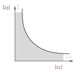
Figure \PageIndex{1}
Find the domain of convergence of \sum_{j,k} \frac{1}{k!} z_1^jz_2^k and draw the corresponding picture.
Find the domain of convergence of \sum_{j,k} c_{j,k} z_1^jz_2^k and draw the corresponding picture if c_{k,k} = 2^k, c_{0,k} = c_{j,0} = 1 and c_{j,k} = 0 otherwise.
Suppose a power series in two variables can be written as a sum of a power series in z_1 and a power series in z_2. Show that the domain of convergence is a polydisc.
Suppose U \subset \mathbb{C}^n is a domain such that if z \in U and |z_k| = |w_k| for all k, then w \in U. Such a U is called a Reinhardt domain. The domains we were drawing so far are Reinhardt domains. They are exactly the domains that you can draw by plotting what happens for the moduli of the variables. A domain is called a complete Reinhardt domain if whenever z \in U, then for r = (r_1,\ldots,r_n) where r_k = |z_k| for all k, we have that the whole polydisc \overline{\Delta_r(0)} \subset U. So a complete Reinhardt domain is a union (possibly infinite) of polydiscs centered at the origin.
Let W \subset \mathbb{C}^n be the set where a certain power series at the origin converges. Show that the interior of W is a complete Reinhardt domain.
Identity Theorem
Let U \subset \mathbb{C}^n be a domain (connected open set) and let f \colon U \to \mathbb{C} be holomorphic. If f|_N \equiv 0 for a nonempty open subset N \subset U, then f \equiv 0.
- Proof
-
Let Z be the set where all derivatives of f are zero; then N \subset Z, so Z is nonempty. The set Z is closed in U as all derivatives are continuous. Take an arbitrary a \in Z. Expand f in a power series around a converging to f in a polydisc \Delta_\rho(a) \subset U. As the coefficients are given by derivatives of f, the power series is the zero series. Hence, f is identically zero in \Delta_\rho(a). Therefore, Z is open. As Z is also closed and nonempty, and U is connected, we have Z = U.
The theorem is often used to show that if two holomorphic functions f and g are equal on a small open set, then f \equiv g.
Maximum Principle
Let U \subset \mathbb{C}^n be a domain. Let f \colon U \to \mathbb{C} be holomorphic and suppose |f(z)| attains a local maximum at some a \in U. Then f \equiv f(a).
- Proof
-
Suppose |f(z)| attains a local maximum at a \in U. Consider a polydisc \Delta = \Delta_1 \times \cdots \times \Delta_n \subset U centered at a. The function z_1 \mapsto f(z_1,a_2,\ldots,a_n) is holomorphic on the disc \Delta_1 and its modulus attains the maximum at the center. Therefore, it is constant by maximum principle in one variable, that is, f(z_1,a_2,\ldots,a_n) = f(a) for all z_1 \in \Delta_1. For any fixed z_1 \in \Delta_1, consider the function z_2 \mapsto f(z_1,z_2,a_3,\ldots,a_n) . This function, holomorphic on the disc \Delta_2, again attains its maximum modulus at the center of \Delta_2 and hence is constant on \Delta_2. Iterating this procedure we obtain that f(z) = f(a) for all z \in \Delta. The identity theorem says that f(z) = f(a) for all z \in U.
Let V be the volume measure on \mathbb{R}^{2n} and hence on \mathbb{C}^n. Suppose \Delta centered at a \in \mathbb{C}^n, and f is a function holomorphic on a neighborhood of \overline{\Delta}. Prove f(a) = \frac{1}{V(\Delta)} \int_{\Delta} f(\zeta) \, dV(\zeta) , where V(\Delta) is the volume of \Delta and dV is the volume measure. That is, f(a) is an average of the values on a polydisc centered at a.
Prove the maximum principle by using the Cauchy formula instead. Hint: Use the previous exercise.
Prove a several variables analogue of the Schwarz's lemma: Suppose f is holomorphic in a neighborhood of \overline{\mathbb{D}^n}, f(0) = 0, and for some k \in \mathbb{N} we have \frac{\partial^{|\alpha|} f}{\partial z^\alpha} (0) = 0 whenever |\alpha| < k. Further suppose for all z \in \mathbb{D}^n, |f(z)| \leq M for some M. Show that |f(z)| \leq M ||z||^k \qquad \text{for all $z \in \overline{\mathbb{D}^n}$}.
Apply the one-variable Liouville’s theorem to prove it for several variables. That is, suppose f \colon \mathbb{C}^n \to \mathbb{C} is holomorphic and bounded. Prove f is constant.
Improve Liouville’s theorem slightly in \mathbb{C}^2. A complex line though the origin is the image of a linear map L \colon \mathbb{C} \to \mathbb{C}^n.
- Prove that for any collection of finitely many complex lines through the origin, there exists an entire nonconstant holomorphic function (n \geq 2) bounded (hence constant) on these complex lines.
- Prove that if an entire holomorphic function in \mathbb{C}^2 is bounded on countably many distinct complex lines through the origin, then it is constant.
- Find a nonconstant entire holomorphic function in \mathbb{C}^3 that is bounded on countably many distinct complex lines through the origin.
Prove the several variables version of Montel's theorem: Suppose \{ f_k \} is a uniformly bounded sequence of holomorphic functions on an open set U \subset \mathbb{C}^n. Show that there exists a subsequence \{ f_{k_j} \} that converges uniformly on compact subsets to some holomorphic function f. Hint: Mimic the one-variable proof.
Prove a several variables version of Hurwitz's theorem: Suppose \{ f_k \} is a sequence of nowhere zero holomorphic functions on a domain U \subset \mathbb{C}^n converging uniformly on compact subsets to a function f. Show that either f is identically zero, or that f is nowhere zero. Hint: Feel free to use the one-variable result.
Suppose p \in \mathbb{C}^n is a point and D \subset \mathbb{C}^n is a ball centered at p \in D. A holomorphic function f \colon D \to \mathbb{C} can be analytically continued along a path \gamma \colon [0,1] \to \mathbb{C}^n, \gamma(0) = p, if for every t \in [0,1] there exists a ball D_t centered at \gamma(t), where D_0 = D, and a holomorphic function f_t \colon D_t \to \mathbb{C}, where f_0 = f, and for each t_0 \in [0,1] there is an \epsilon > 0 such that if |t-t_0| < \epsilon, then f_t = f_{t_0} in D_t \cap D_{t_0}. Prove a several variables version of the Monodromy theorem: If U \subset \mathbb{C}^n is a simply connected domain, D \subset U a ball and f \colon D \to \mathbb{C} a holomorphic function that can be analytically continued from p \in D to every q \in U, then there exists a unique holomorphic function F \colon U \to \mathbb{C} such that F|_D = f.
The set of holomorphic functions on a domain is a commutative ring under pointwise addition and multiplication (exercise below). We give this set a name.
Let U \subset \mathbb{C}^n be an open set. Define \mathcal{O}(U) to be the ring of holomorphic functions. The letter \mathcal{O} is used to recognize the fundamental contribution to several complex variables by Kiyoshi Oka^{1}.
Prove that \mathcal{O}(U) is actually a commutative ring with the operations (f+g)(z) = f(z)+g(z), \qquad (fg)(z) = f(z)g(z) .
Show that \mathcal{O}(U) is an (has no zero divisors) if and only if U is connected. That is, show that U being connected is equivalent to showing that if h(z) = f(z)g(z) is identically zero for f,g \in \mathcal{O}(U), then either f or g is identically zero.
A function F defined on a dense open subset of U is meromorphic if locally near every p \in U, F = \frac{f}{g} for f and g holomorphic in some neighborhood of p. It is from a deep result of Oka that for domains U \subset \mathbb{C}^n, every meromorphic function can be represented as \frac{f}{g} globally. That is, the ring of meromorphic functions is the field of fractions of \mathcal{O}(U). This problem is the so-called Poincaré problem, and its solution is no longer positive once we generalize U to complex manifolds. The points of U through which F does not extend holomorphically are called the poles of F. Namely, poles are the points where g=0 for every possible representation \frac{f}{g}. Unlike in one variable, in several variables poles are never isolated points. There is also a new type of singular point for meromorphic functions in more than one variable:
In two variables one can no longer think of a meromorphic function F having the value \infty when the denominator vanishes. Show that F(z,w) = \frac{z}{w} achieves all values of \mathbb{C} in every neighborhood of the origin. We call the origin a point of indeterminacy.
Prove that zeros (and so poles as we will see later, though this is a bit harder to see) are never isolated in \mathbb{C}^n for n \geq 2. Hint: Consider z_1 \mapsto f(z_1,z_2,\ldots,z_n) as you move z_2,\ldots,z_n around, and use perhaps Hurwitz.