
2.2: Tangent Vectors, the Hessian, and Convexity
- Page ID
- 74229

An exercise in the previous section showed that every convex domain is a domain of holomorphy. However, classical convexity is too strong.
Show that if \(U \subset \mathbb{C}^m\) and \(V \subset \mathbb{C}^k\) are both domains of holomorphy, then \(U \times V\) is a domain of holomorphy.
In particular, the exercise says that for any domains \(U \subset \mathbb{C}\) and \(V \subset \mathbb{C}\), the set \(U \times V\) is a domain of holomorphy in \(\mathbb{C}^2\). The domains \(U\) and \(V\), and hence \(U \times V\), can be spectacularly nonconvex. But we should not discard convexity completely, there is a notion of pseudoconvexity, which vaguely means “convexity in the complex directions” and is the correct notion to distinguish domains of holomorphy. Let us figure out what classical convexity means locally for a smooth boundary.
A set \(M \subset \mathbb{R}^n\) is a \(C^k\)-smooth hypersurface if at each point \(p \in M\), there exists a \(k\)-times continuously differentiable function \(r \colon V \to \mathbb{R}\) with nonvanishing derivative, defined in a neighborhood \(V\) of \(p\) such that \(M \cap V = \bigl\{ x \in V : r(x) = 0 \bigr\}\). The function \(r\) is called the defining function of \(M\) (at \(p\)).
An open set (or domain) \(U \subset \mathbb{R}^n\) with \(C^k\)-smooth boundary is a set where \(\partial U\) is a \(C^k\)-smooth hypersurface, and at every \(p \in \partial U\) there is a defining function \(r\) such that \(r < 0\) for points in \(U\) and \(r > 0\) for points not in \(U\). See .
If we say simply smooth, we mean \(C^\infty\)-smooth, that is, the \(r\) above is infinitely differentiable.
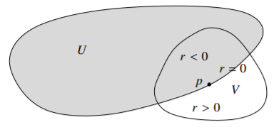
Figure \(\PageIndex{1}\)
What we really defined is an embedded hypersurface. In particular, in this book the topology on the set \(M\) will be the subset topology. Furthermore, in this book we generally deal with smooth (that is, \(C^\infty\)) functions and hypersurfaces. Dealing with \(C^k\)-smooth functions for finite \(k\) introduces technicalities that make certain theorems and arguments unnecessarily difficult.
As the derivative of \(r\) is nonvanishing, a hypersurface \(M\) is locally the graph of one variable over the rest using the implicit function theorem. That is, \(M\) is a smooth hypersurface if it is locally a set defined by \(x_j = \varphi(x_1,\ldots,x_{j-1},x_{j+1},\ldots,x_n)\) for some \(j\) and some smooth function \(\varphi\).
The definition of an open set with smooth boundary is not just that the boundary is a smooth hypersurface, that is not enough. It also says that one side of that hypersurface is in \(U\) and one side is not in \(U\). That is because if the derivative of \(r\) never vanishes, then \(r\) must have different signs on different sides of \(\bigl\{ x \in V : r(x) = 0 \bigr\}\). The verification of this fact is left to the reader. (Hint: Look at where the gradient points to.)
Same definition works for \(\mathbb{C}^n\), where we treat \(\mathbb{C}^n\) as \(\mathbb{R}^{2n}\). For example, the ball \(\mathbb{B}_{n}\) is a domain with smooth boundary with defining function \(r(z,\bar{z}) = ||z||^2-1\). We can, in fact, find a single global defining function for every open set with smooth boundary, but we have no need of this. In \(\mathbb{C}^n\) a hypersurface defined as above is a real hypersurface, to distinguish it from a complex hypersurface that would be the zero set of a holomorphic function, although we may at times leave out the word “real” if it is clear from context.
For a point \(p \in \mathbb{R}^n\), the set of tangent vectors \(T_p \mathbb{R}^n\) is given by \[T_p \mathbb{R}^n = \operatorname{span}_{\mathbb{R}} \left\{ \frac{\partial}{\partial x_1}\Big|_p, \ldots, \frac{\partial}{\partial x_n}\Big|_p \right\} .\]
That is, a vector \(X_p \in T_p \mathbb{R}^n\) is an object of the form \[X_p = \sum_{j=1}^n a_j \frac{\partial}{\partial x_j}\Big|_p ,\] for real numbers \(a_j\). For computations, \(X_p\) could be represented by an \(n\)-vector \(a = (a_1,\ldots,a_n)\). However, if \(p \not= q\), then \(T_p \mathbb{R}^n\) and \(T_q \mathbb{R}^n\) are distinct spaces. An object \(\frac{\partial}{\partial x_j}\big|_p\) is a linear functional on the space of smooth functions: When applied to a smooth function \(g\), it gives \(\frac{\partial g}{\partial x_j} \big|_p\). Therefore, \(X_p\) is also such a functional. It is the directional derivative from calculus; it is computed as \(X_p f = \nabla f|_p \cdot (a_1,\ldots,a_n)\).
Let \(M \subset \mathbb{R}^n\) be a smooth hypersurface, \(p \in M\), and \(r\) is a defining function at \(p\), then a vector \(X_p \in T_p \mathbb{R}^n\) is tangent to \(M\) at \(p\) if \[X_p r = 0, \qquad \text{or in other words} \qquad \sum_{j=1}^n a_j \frac{\partial r}{\partial x_j} \Big|_p = 0 .\] The space of tangent vectors to \(M\) is denoted by \(T_p M\), and is called the tangent space to \(M\) at \(p\).
The space \(T_pM\) is an \((n-1)\)-dimensional real vector space—it is a subspace of an \(n\)-dimensional \(T_p\mathbb{R}^n\) given by a single linear equation. Recall from calculus that the gradient \(\nabla r|_p\) is “normal” to \(M\) at \(p\), and the tangent space is given by all the \(n\)-vectors \(a\) that are orthogonal to the normal, that is, \(\nabla r|_p \cdot a = 0\).
We cheated in the terminology, and assumed without justification that \(T_pM\) depends only on \(M\), not on \(r\). Fortunately, the definition of \(T_pM\) is independent of the choice of \(r\) by the next two exercises.
Suppose \(M \subset \mathbb{R}^n\) is a smooth hypersurface and \(r\) is a smooth defining function for \(M\) at \(p\).
- Suppose \(\varphi\) is another smooth defining function of \(M\) on a neighborhood of \(p\). Show that there exists a smooth nonvanishing function \(g\) such that \(\varphi = g r\) (in a neighborhood of \(p\)).
- Now suppose \(\varphi\) is an arbitrary smooth function that vanishes on \(M\) (not necessarily a defining function). Again show that \(\varphi = g r\), but now \(g\) may possibly vanish.
Hint: First suppose \(r=x_n\) and find a \(g\) such that \(\varphi = x_n g\). Then find a local change of variables to make \(M\) into the set given by \(x_n = 0\). A useful calculus fact: If \(f(0) = 0\) and \(f\) is smooth, then \(s \int_0^1 f'(ts) \,dt = f(s)\), and \(\int_0^1 f'(ts) \,dt\) is a smooth function of \(s\).
Show that \(T_pM\) is independent of which defining function we take. That is, prove that if \(r\) and \(\tilde{r}\) are defining functions for \(M\) at \(p\), then \(\sum_j a_j \frac{\partial r}{\partial x_j} \big|_p = 0\) if and only if \(\sum_j a_j \frac{\partial \tilde{r}}{\partial x_j} \big|_p = 0\).
The tangent space \(T_p M\) is the set of derivatives along \(M\) at \(p\). If \(r\) is a defining function of \(M\), and \(f\) and \(h\) are two smooth functions such that \(f=h\) on \(M\), then Exercise \(\PageIndex{2}\) says that \[f-h = g r, \qquad \text{or} \qquad f = h + g r,\] for some smooth \(g\). Applying \(X_p\) we find \[X_p f = X_p h + X_p (gr) = X_p h + (X_p g)r + g(X_p r) = X_p h + (X_p g)r.\] So \(X_p f = X_p h\) on \(M\) (where \(r=0\)). In other words, \(X_p f\) only depends on the values of \(f\) on \(M\).
If \(M \subset \mathbb{R}^n\) is given by \(x_n = 0\), then \(T_p M\) is given by derivatives of the form \[X_p = \sum_{j=1}^{n-1} a_j \frac{\partial}{\partial x_j} \Big|_p .\] That is, derivatives along the first \(n-1\) variables only.
The disjoint union \[T\mathbb{R}^n = \bigcup_{p \in \mathbb{R}^n} T_p \mathbb{R}^n\] is called the tangent bundle. There is a natural identification \(\mathbb{R}^n \times \mathbb{R}^n \cong T\mathbb{R}^n\): \[(p,a) \in \mathbb{R}^n \times \mathbb{R}^n \quad \mapsto \quad \sum_{j=1}^n a_j \frac{\partial}{\partial x_j} \Big|_p \in T\mathbb{R}^n .\] The topology and smooth structure on \(T\mathbb{R}^n\) comes from this identification. The wording “bundle” (a bundle of fibers) comes from the natural projection \(\pi \colon T\mathbb{R}^n \to \mathbb{R}^n\), where fibers are \(\pi^{-1}(p) = T_p\mathbb{R}^n\).
A smooth vector field in \(T\mathbb{R}^n\) is an object of the form \[X = \sum_{j=1}^n a_j \frac{\partial}{\partial x_j} ,\] where \(a_j\) are smooth functions. That is, \(X\) is a smooth function \(X \colon V \subset \mathbb{R}^n \to T\mathbb{R}^n\) such that \(X(p) \in T_p \mathbb{R}^n\). Usually we write \(X_p\) rather than \(X(p)\). To be more fancy, say \(X\) is a section of \(T \mathbb{R}^n\).
Similarly, the tangent bundle of \(M\) is \[TM = \bigcup_{p \in M} T_p M .\] A vector field \(X\) in \(TM\) is a vector field such that \(X_p \in T_p M\) for all \(p \in M\).
Before we move on, let us note how smooth maps transform tangent spaces. Given a smooth mapping \(f \colon U \subset \mathbb{R}^n \to \mathbb{R}^m\), the derivative at \(p\) is a linear mapping of the tangent spaces: \(Df(p) \colon T_p \mathbb{R}^n \to T_{f(p)} \mathbb{R}^m\). If \(X_p \in T_p \mathbb{R}^n\), then \(Df(p) X_p\) should be in \(T_{f(p)} \mathbb{R}^m\). The vector \(Df(p) X_p\) is defined by how it acts on smooth functions \(\varphi\) of a neighborhood of \(f(p)\) in \(\mathbb{R}^m\): \[Df(p) X_p \varphi = X_p (\varphi \circ f) .\] It is the only reasonable way to put those three objects together. When the spaces are \(\mathbb{C}^n\) and \(\mathbb{C}^m\), we denote this derivative as \(D_\mathbb{R} f\) to distinguish it from the holomorphic derivative. As far as calculus computations are concerned, the linear mapping \(Df(p)\) is the Jacobian matrix acting on vectors in the standard basis of the tangent space as given above. This is why we use the same notation for the Jacobian matrix and the derivative acting on tangent spaces. To verify this claim, it is enough to see where the basis element \(\frac{\partial}{\partial x_j}\big|_p\) goes, and the form of \(Df(p)\) as a matrix follows by the chain rule. For example, the derivative of the mapping \(f(x_1,x_2) = (x_1+2x_2+x_1^2,3x_1+4x_2+x_1x_2)\) at the origin is given by the matrix \(\left[ \begin{smallmatrix} 1 & 2 \\ 3 & 4 \end{smallmatrix} \right]\), and so the vector \(X_p = a\frac{\partial}{\partial x_1}\big|_0 + b\frac{\partial}{\partial x_2}\big|_0\) gets taken to \(Df(0) X_0 = (a+2b)\frac{\partial}{\partial y_1}\big|_0 + (3a+4b)\frac{\partial}{\partial y_2}\big|_0\), where we let \((y_1,y_2)\) be the coordinates on the target. You should check on some test function, such as \(\varphi(y_1,y_2) = \alpha y_1 + \beta y_2\), that the definition above is satisfied.
Now that we know what tangent vectors are and how they transform, let us define convexity for domains with smooth boundary.
Suppose \(U \subset \mathbb{R}^n\) is an open set with smooth boundary, and \(r\) is a defining function for \(\partial U\) at \(p \in \partial U\) such that \(r < 0\) on \(U\). If \[\sum_{j=1,\ell=1}^n a_j a_\ell \frac{\partial^2 r}{\partial x_j \partial x_\ell} \Big|_p \geq 0 , \qquad \text{for all} \qquad X_p = \sum_{j=1}^n a_j \frac{\partial}{\partial x_j}\Big|_p \quad \in \quad T_p \partial U,\] then \(U\) is said to be convex at \(p\). If the inequality above is strict for all nonzero \(X_p \in T_p \partial U\), then \(U\) is said to be strongly convex at \(p\).
A domain \(U\) is convex if it is convex at all \(p \in \partial U\). If \(U\) is bounded\(^{1}\), we say \(U\) is strongly convex if it is strongly convex at all \(p \in \partial U\).
The matrix \[\left[ \frac{\partial^2 r}{\partial x_j \partial x_\ell} \Big|_p \right]_{j\ell}\] is the Hessian of \(r\) at \(p\). So, \(U\) is convex at \(p \in \partial U\) if the Hessian of \(r\) at \(p\) as a bilinear form is positive semidefinite when restricted to \(T_p \partial U\). In the language of vector calculus, let \(H\) be the Hessian of \(r\) at \(p\), and treat \(a \in \mathbb{R}^n\) as a column vector. Then \(\partial U\) is convex at \(p\) whenever \[a^t H a \geq 0 , \qquad \text{for all $a \in \mathbb{R}^n$ such that} \quad \nabla r|_p \cdot a = 0 .\] This bilinear form given by the Hessian is the second fundamental form from Riemannian geometry in mild disguise (or perhaps it is the other way around).
We cheated a little bit, since we have not proved that the notion of convexity is well-defined. In particular, there are many possible defining functions.
Show that the definition of convexity is independent of the defining function. Hint: If \(\tilde{r}\) is another defining function near \(p\), then there is a smooth function \(g > 0\) such that \(\tilde{r} = g r\).
The unit disc in \(\mathbb{R}^2\) is convex (actually strongly convex). Proof: Let \((x,y)\) be the coordinates and let \(r(x,y) = x^2+y^2-1\) be the defining function.
The tangent space of the circle is one-dimensional, so we simply need to find a single nonzero tangent vector at each point. Consider the gradient \(\nabla r = (2x,2y)\) to check that \[X = y \frac{\partial}{\partial x} - x \frac{\partial}{\partial y}\] is tangent to the circle, that is, \(Xr = X(x^2+y^2-1) = (2x,2y) \cdot (y,-x) = 0\) on the circle (by chance \(Xr=0\) everywhere). The vector field \(X\) is nonzero on the circle, so at each point it gives a basis of the tangent space. See Figure \(\PageIndex{2}\).
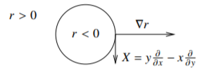
Figure \(\PageIndex{2}\)
The Hessian matrix of \(r\) is \[\begin{bmatrix} \frac{\partial^2 r}{\partial x^2} & \frac{\partial^2 r}{\partial x \partial y} \\ \frac{\partial^2 r}{\partial y \partial x} & \frac{\partial^2 r}{\partial y^2} \end{bmatrix} = \begin{bmatrix} 2 & 0 \\ 0 & 2 \end{bmatrix} .\] Applying the vector \((y,-x)\) gets us \[\begin{bmatrix} y & -x \end{bmatrix} \begin{bmatrix} 2 & 0 \\ 0 & 2 \end{bmatrix} \begin{bmatrix} y \\ -x \end{bmatrix} = 2y^2+2x^2 = 2 > 0 .\] So the domain given by \(r < 0\) is strongly convex at all points.
In general, to construct a tangent vector field for a curve in \(\mathbb{R}^2\), consider \(r_y \frac{\partial}{\partial x} - r_x \frac{\partial}{\partial y}\). In higher dimensions, running through enough pairs of variables gets a basis of \(TM\).
Show that if an open set with smooth boundary is strongly convex at a point, then it is strongly convex at all nearby points. On the other hand find an example of an open set with smooth boundary that is convex at one point \(p\), but not convex at points arbitrarily near \(p\).
Show that the domain in \(\mathbb{R}^2\) defined by \(x^4+y^4 < 1\) is convex, but not strongly convex. Find all the points where the domain is not strongly convex.
Show that the domain in \(\mathbb{R}^3\) defined by \({(x_1^2+x_2^2)}^2 < x_3\) is strongly convex at all points except the origin, where it is just convex (but not strongly).
In the following, we use the big-oh notation, although we use a perhaps less standard shorthand\(^{2}\). A smooth function is \(O(\ell)\) at a point \(p\) (usually the origin), if all its derivatives of order \(0, 1, \ldots, \ell-1\) vanish at \(p\). For example, if \(f\) is \(O(3)\) at the origin, then \(f(0)=0\), and its first and second derivatives vanish at the origin.
For computations it is often useful to use a more convenient defining function, that is, it is convenient to write \(M\) as a graph.
Suppose \(M \subset \mathbb{R}^n\) is a smooth hypersurface, and \(p \in M\). Then after a rotation and translation, \(p\) is the origin, and near the origin \(M\) is given by \[y = \varphi(x) ,\] where \((x,y) \in \mathbb{R}^{n-1} \times \mathbb{R}\) are our coordinates and \(\varphi\) is a smooth function that is \(O(2)\) at the origin, namely, \(\varphi(0) = 0\) and \(d\varphi(0) = 0\).
If \(M\) is the boundary of an open set \(U\) with smooth boundary and \(r < 0\) on \(U\), then the rotation can be chosen such that \(y > \varphi(x)\) for points in \(U\). See Figure \(\PageIndex{3}\).
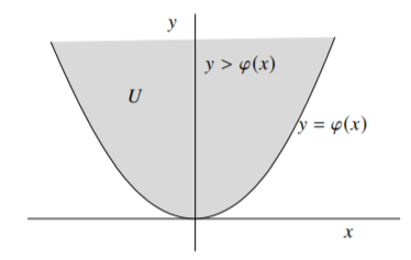
Figure \(\PageIndex{3}\)
- Proof
-
Let \(r\) be a defining function at \(p\). Take \(v = \nabla r|_p\). By translating \(p\) to zero, and applying a rotation (an orthogonal matrix), we assume \(v = (0,0,\ldots,0,v_n)\), where \(v_n < 0\). Denote our coordinates by \((x,y) \in \mathbb{R}^{n-1} \times \mathbb{R}\). As \(\nabla r|_0 = v\), then \(\frac{\partial r}{\partial y}(0) \not= 0\). We apply the implicit function theorem to find a smooth function \(\varphi\) such that \(r\bigl(x,\varphi(x)\bigr) = 0\) for all \(x\) in a neighborhood of the origin, and \(\bigl\{ (x,y) : y=\varphi(x) \bigr\}\) are all the solutions to \(r = 0\) near the origin.
What is left is to show that the derivative at 0 of \(\varphi\) vanishes. As \(r\bigl(x,\varphi(x)\bigr) = 0\) for all \(x\) in a neighborhood of the origin, we differentiate. For every \(j=1,\ldots,n-1\), \[0 = \frac{\partial}{\partial x_j} \Bigl[ r\bigl(x,\varphi(x)\bigr) \Bigr] = \left( \sum_{\ell=1}^{n-1} \frac{\partial r}{\partial x_\ell} \frac{\partial x_\ell}{\partial x_j} \right) + \frac{\partial r}{\partial y} \frac{\partial \varphi}{\partial x_j} = \frac{\partial r}{\partial x_j} + \frac{\partial r}{\partial y} \frac{\partial \varphi}{\partial x_j} .\] At the origin, \(\frac{\partial r}{\partial x_j}(0,0) = 0\) and \(\frac{\partial r}{\partial y}(0,0) = v_n \not= 0\), and therefore \(\frac{\partial \varphi}{\partial x_j}(0) = 0\).
To prove the final statement, note that \(r < 0\) on \(U\). It is enough to check that \(r\) is negative for \((0,y)\) if \(y > 0\) is small, which follows as \(\frac{\partial r}{\partial y}(0,0) = v_n < 0\).
The advantage of this representation is that the tangent space at \(p\) can be identified with the \(x\) coordinates for the purposes of computation. Considering \(x\) as a column vector, the Taylor expansion of a smooth function \(\varphi\) at the origin is \[\varphi(x) = \varphi(0) + \nabla \varphi|_0 \cdot x + \frac{1}{2}\, x^t H x + E(x) ,\] where \(H = \left[ \frac{\partial^2 \varphi}{\partial x_j \partial x_k} \big|_{0} \right]_{jk}\) is the Hessian matrix of \(\varphi\) at the origin, and \(E\) is \(O(3)\), namely, \(E(0) = 0\), and all first and second order derivatives of \(E\) vanish at \(0\). For the situation of the lemma above, the \(\varphi\) is \(O(2)\) at the origin, i.e. \(\varphi(0) = 0\) and \(\nabla \varphi|_0 = 0\). So we write the hypersurface \(M\) as \[y = \frac{1}{2}\, x^t H x + E(x) .\] If \(M\) is the boundary \(\partial U\) of an open set, then we pick the rotation so that \(y > \frac{1}{2}\,x^t H x + E(x)\) on \(U\). It is an easy exercise to show that \(U\) is convex at \(p\) if \(H\) positive semidefinite, and \(U\) is strongly convex at \(p\) if \(H\) is positive definite.
Prove the statement above about \(H\) and convexity at \(p\).
Let \(r\) be a defining function at \(p\) for a smooth hypersurface \(M \subset \mathbb{R}^n\). We say \(M\) is convex from both sides at \(p\) if both the set given by \(r > 0\) and the set given by \(r < 0\) are convex at \(p\). Prove that if a hypersurface \(M \subset \mathbb{R}^n\) is convex from both sides at all points, then it is locally just a hyperplane (the zero set of a real affine function).
Recall that \(U\) is geometrically convex if for every \(p,q \in U\) the line between \(p\) and \(q\) is in \(U\), or in other words \(tp +(1-t)q \in U\) for all \(t \in [0,1]\). In particular, geometric convexity is a global condition. You need to know all of \(U\). On the other hand, the notion of convex for a smooth boundary is local in that you only need to know \(\partial U\) in a small neighborhood. For domains with smooth boundaries the two notions are equivalent. Proving one direction is easy.
Suppose a domain \(U \subset \mathbb{R}^n\) with smooth boundary is geometrically convex. Show that it is convex.
The other direction is considerably more complicated, and we will not worry about it here. Proving a global condition from a local one is often trickier, but also often more interesting. Similar difficulties will be present once we move back to several complex variables and try to relate pseudoconvexity with domains of holomorphy.