5.3: Graphs and Properties of Exponential Growth and Decay Functions

Learning Objectives

In this section, you will:

1. Examine properties of exponential functions
2. Examine graphs of exponential functions

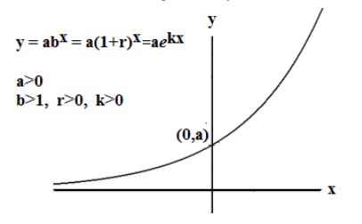
An exponential function can be written in forms

\[f(x) = ab^x = a(1 + r)^x = ae^{kx} \nonumber \]

where

• \(\mathbf{a}\) is the initial value because \(f(0) = a\). In the growth and decay models that we examine in this finite math textbook, \(a > 0\).
• \(\mathbf{b}\) is often called the growth factor. We restrict \(b\) to be positive (\(b > 0\)) because even roots of negative numbers are undefined. We want the function to be defined for all values of \(x\), but \(b^x\) would be undefined for some values of \(x\) if \(b<0\).
• \(\mathbf{r}\) is called the growth or decay rate. In the formula for the functions, we use r in decimal form, but in the context of a problem we usually state r as a percent.
• \(\mathbf{k}\) is called the continuous growth rate or continuous decay rate.

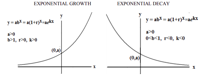
Properties of Exponential Growth Functions

The function \(y=f(x) = ab^x\) represents growth if \(b > 1\) and \(a > 0\).

The growth rate \(r\) is positive when \(b>1\). Because \(b = 1+ r > 1\), then \(r = b−1 > 0\)

The function \(y=f(x) = ae^{kx}\) represents growth if \(k > 0\) and \(a > 0\).

The function is an increasing function; \(y\) increases as \(x\) increases.

• Domain: { all real numbers} ; all real numbers can be input to an exponential function
• Range: If \(a>0\), the range is {positive real numbers} The graph is always above the x axis.
• Horizontal Asymptote: when \(b > 1\), the horizontal asymptote is the negative x axis, as x becomes large negative. Using mathematical notation: as x → −∞, then y → 0.
• The vertical intercept is the point \((0,a)\) on the y-axis. There is no horizontal intercept because the function does not cross the x-axis.

Properties of Exponential Decay Functions

The function \(y=f(x) = ab^x\) function represents decay if \(0 < b < 1\) and \(a > 0\).

The growth rate \(r\) is negative when \(0 < b < 0\). Because \(b=1+r < 1\), then \(r=b-1<0\).

The function \(y=f(x) = ae^{kx}\) function represents decay if \(k < 0\) and \(a > 0\).

The function is a decreasing function; \(y\) decreases as \(x\) increases.

Domain: { all real numbers} ; all real numbers can be input to an exponential function

Range: If \(a>0\), the range is { positive real numbers } The graph is always above the x axis.

Horizontal Asymptote: when \(b < 1\), the horizontal asymptote is the positive x axis as x becomes large positive. Using mathematical notation: as x → ∞, then y → 0.

The vertical intercept is the point \((0,a)\) on the y-axis. There is no horizontal intercept because the function does not cross the x-axis.

The graphs for exponential growth and decay functions are displayed below for comparison.

An Exponential Function is a One-to-One Function

Observe that in the graph of an exponential function, each y value on the graph occurs only once. Therefore, every y value in the range corresponds to only one x value. So, for any particular value of y, you can use the graph to see which value of x is the input to produce that y value as output. This property is called “one-to-one”.

Because for each value of the output y, you can uniquely determine the value of the corresponding input x, thus every exponential function has an inverse function. The inverse function of an exponential function is a logarithmic function, which we will investigate in the next section.

Example \(\PageIndex{1}\)

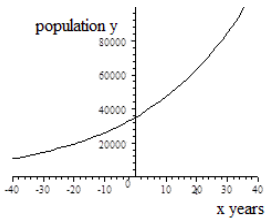
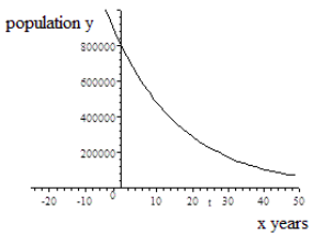
\(x\) years after the year 2015, the population of the city of Fulton is given by the function \(y= f(x) = 35000(1.03^x)\). \(x\) years after the year 2015, the population of the city of Greenville is given by the function \(y = g(x) = 80000(0.95^x)\). Compare the graphs of these functions.

Solution

The graphs below were created using computer graphing software. You can also graph these functions using a graphing calculator.

Population of Fulton	Population of Greenville
\[y=f(x)=35000\left(1.03^{x}\right) \nonumber \]	\[y=g(x)=80000\left(0.95^{x}\right) \nonumber \]
Fulton's population is increasing. \(b = 1.03 > 1\) and \(r=0.03>0\) Exponential Growth	Greenville’s population is decreasing. \(b = 0.95 < 1\) and \(r = −0.05 < 0\) Exponential Decay
y-intercept: (0, 35000) The initial population in 2015 is 35000.	y-intercept: (0,80000) The initial population in 2015 is 80000.
Horizontal Asymptote: The negative x axis is the horizontal asymptote. y → 0 as x → − ∞	Horizontal Asymptote: The positive x axis is the horizontal asymptote. y → 0 as x → ∞

Domain: In general, the domain of both functions \(y= f(x) = 35000(1.03^x)\) and \(y= g(x) = 80000(0.95^x)\) is the set of all real numbers.

Range: The range of both functions is the set of positive real numbers. Both graphs always lie above the x-axis.

Domain and Range in context of this problem:

The functions represent population size as a function of time after the year 2015 . We restrict the domain in this context, using the “practical domain” as the set of all non-negative real numbers: \(x≥0\). Then we would consider only the portion of the graph that lies in the first quadrant.

• If we restrict the domain to \(x≥0\) for the growth function \(y= f(x) = 35000(1.03^x)\), then the range for the population of Fulton is \(y ≥ 35,000\)
• If we restrict the domain to \(x≥0\) for the decay function \(y= g(x) = 80000(0.95^x)\), then the range for the population of Greenville is \(y ≤ 80,000\).