10.1: Introduction to Markov Chains

Last updated
Save as PDF

Page ID: 37930

$ \newcommand{\vecs}[1]{\overset { \scriptstyle \rightharpoonup} {\mathbf{#1}} } $ $ \newcommand{\vecd}[1]{\overset{-\!-\!\rightharpoonup}{\vphantom{a}\smash {#1}}} $$\newcommand{\id}{\mathrm{id}}$ $ \newcommand{\Span}{\mathrm{span}}$ $ \newcommand{\kernel}{\mathrm{null}\,}$ $ \newcommand{\range}{\mathrm{range}\,}$ $ \newcommand{\RealPart}{\mathrm{Re}}$ $ \newcommand{\ImaginaryPart}{\mathrm{Im}}$ $ \newcommand{\Argument}{\mathrm{Arg}}$ $ \newcommand{\norm}[1]{\| #1 \|}$ $ \newcommand{\inner}[2]{\langle #1, #2 \rangle}$ $ \newcommand{\Span}{\mathrm{span}}$ $\newcommand{\id}{\mathrm{id}}$ $ \newcommand{\Span}{\mathrm{span}}$ $ \newcommand{\kernel}{\mathrm{null}\,}$ $ \newcommand{\range}{\mathrm{range}\,}$ $ \newcommand{\RealPart}{\mathrm{Re}}$ $ \newcommand{\ImaginaryPart}{\mathrm{Im}}$ $ \newcommand{\Argument}{\mathrm{Arg}}$ $ \newcommand{\norm}[1]{\| #1 \|}$ $ \newcommand{\inner}[2]{\langle #1, #2 \rangle}$ $ \newcommand{\Span}{\mathrm{span}}$$\newcommand{\AA}{\unicode[.8,0]{x212B}}$

Learning Objectives

In this chapter, you will learn to:

Write transition matrices for Markov Chain problems.
Use the transition matrix and the initial state vector to find the state vector that gives the distribution after a specified number of transitions.

We will now study stochastic processes, experiments in which the outcomes of events depend on the previous outcomes; stochastic processes involve random outcomes that can be described by probabilities. Such a process or experiment is called a Markov Chain or Markov process. The process was first studied by a Russian mathematician named Andrei A. Markov in the early 1900s.

About 600 cities worldwide have bike share programs. Typically a person pays a fee to join a the program and can borrow a bicycle from any bike share station and then can return it to the same or another system. Each day, the distribution of bikes at the stations changes, as the bikes get returned to different stations from where they are borrowed.

For simplicity, let’s consider a very simple bike share program with only 3 stations: A, B, C. Suppose that all bicycles must be returned to the station at the end of the day, so that each day there is a time, let’s say midnight, that all bikes are at some station, and we can examine all the stations at this time of day, every day. We want to model the movement of bikes from midnight of a given day to midnight of the next day. We find that over a 1 day period,

of the bikes borrowed from station A, 30% are returned to station A, 50% end up at station B, and 20% end up at station C.
of the bikes borrowed from station B, 10% end up at station A, 60% have been returned to station B, and 30% end up at station C
of the bikes borrowed from station C, 10% end up at station A, 10% end up at station B, and 80% are returned to station C.

We can draw an arrow diagram to show this. The arrows indicate the station where the bicycle was started, called its initial state, and the stations at which it might be located one day later, called the terminal states. The numbers on the arrows show the probability for being in each of the indicated terminal states.

$Section10.1.png$

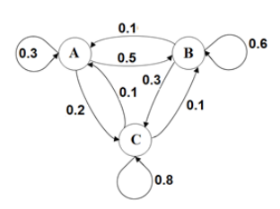
Because our bike share example is simple and has only 3 stations, the arrow diagram, also called a directed graph, helps us visualize the information. But if we had an example with 10, or 20, or more bike share stations, the diagram would become so complicated that it would be difficult to understand the information in the diagram.

We can use a transition matrix to organize the information,

Each row in the matrix represents an initial state. Each column represents a terminal state.
We will assign the rows in order to stations A, B, C, and the columns in the same order to stations A, B, C. Therefore the matrix must be a square matrix, with the same number of rows as columns. The entry in row 2 column 3, for example, would show the probability that a bike that is initially at station B will be at station C one day later: that entry is 0.30, which is the probability in the diagram for the arrow that points from B to C. We use this the letter T for transition matrix.

$Section10.1b.png$

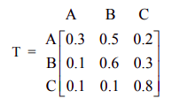
Looking at the first row that represents bikes initially at station A, we see that 30% of the bikes borrowed from station A are returned to station A, 50% end up at station B, and 20% end up at station C, after one day.

We note some properties of the transition matrix:

$t_{ij}$ represents the entry in row $i$ column $j$
$t_{ij}$ = the probability of moving from state represented by row $i$ to the state represented by row $j$ in a single transition

$t_{ij}$ is a conditional probability which we can write as:
$t_{ij}$ = P(next state is the state in column $j$ | current state is the state in row $i$)
Each row adds to 1
All entries are between 0 and 1, inclusive because they are probabilities.
The transition matrix represents change over one transition period; in this example one transition is a fixed unit of time of one day.

Example $\PageIndex{1}$

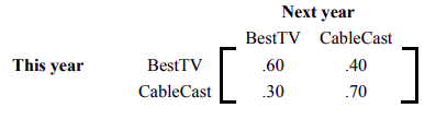
A city is served by two cable TV companies, BestTV and CableCast.

Due to their aggressive sales tactics, each year 40% of BestTV customers switch to CableCast; the other 60% of BestTV customers stay with BestTV.
On the other hand, 30% of the CableCast customers switch to Best TV.

The two states in this example are BestTV and CableCast. Express the information above as a transition matrix which displays the probabilities of going from one state into another state.

Solution

The transition matrix is:

$Example10.1.1.png$

As previously noted, the reader should observe that a transition matrix is always a square matrix because all possible states must have both rows and columns. All entries in a transition matrix are non-negative as they represent probabilities. And, since all possible outcomes are considered in the Markov process, the sum of the row entries is always 1.

With a larger transition matrix, the ideas in Example $\PageIndex{1}$ could be expanded to represent a market with more than 2 cable TV companies. The concepts of brand loyalty and switching between brands demonstrated in the cable TV example apply to many types of products, such as cell phone carriers, brands of regular purchases such as food or laundry detergent, brands major purchases such as cars or appliances, airlines that travelers choose when booking flights, or hotels chains that travelers choose to stay in.

The transition matrix shows the probabilities for transitions between states at two consecutive times. We need a way to represent the distribution among the states at a particular point in time. To do this we use a row matrix called a state vector. The state vector is a row matrix that has only one row; it has one column for each state. The entries show the distribution by state at a given point in time. All entries are between 0 and 1 inclusive, and the sum of the entries is 1.

For the bike share example with 3 bike share stations, the state vector is a $1 \times 3$ matrix with 1 row and 3 columns. Suppose that when we start observing our bike share program, 30% of the bikes are at station A, 45% of the bikes are at station B, and 25% are at station C. The initial state vector is

$Section10.1c.png$

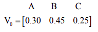
The subscript 0 indicates that this is the initial distribution, before any transitions occur.

If we want to determine the distribution after one transition, we’ll need to find a new state vector that we’ll call V₁. The subscript 1 indicates this is the distribution after 1 transition has occurred.

We find V₁by multiplying V₀by the transitionmatrix T, as follows:

\[\begin{array}{l}
\mathrm{V}_{1}=\mathrm{V}_{0} \mathrm{T} \\
=\left[\begin{array}{lll}
0.30 & 0.45 & 0.25
\end{array}\right]\left[\begin{array}{lll}
0.3 & 0.5 & 0.2 \\
0.1 & 0.6 & 0.3 \\
0.1 & 0.1 & 0.8
\end{array}\right] \\
=[.30(.3)+.45(.1)+.25(.1) \quad .30(.5)+.45(.6)+.25(.1) \quad .30(.2)+.45(.3)+.25(.8)] \\
=\left[\begin{array}{lll}
.16 & .445 & .395
\end{array}\right]
\end{array} \nonumber \]

After 1 day (1 transition), 16 % of the bikes are at station A, 44.5 % are at station B and 39.5% are at station C.

We showed the step by step work for the matrix multiplication above. In the future we’ll generally use technology, such as the matrix capabilities of our calculator, to perform any necessary matrix multiplications, rather than showing the step by step work.

Suppose now that we want to know the distribution of bicycles at the stations after two days. We need to find V₂, the state vector after two transitions. To find V₂ , we multiply the state vector after one transition V₁ by the transition matrix T.

\[\mathrm{V}_{2}=\mathrm{V}_{1} \mathrm{T}=\left[\begin{array}{lll}
.16 & .445 & .395
\end{array}\right]\left[\begin{array}{lll}
0.3 & 0.5 & 0.2 \\
0.1 & 0.6 & 0.3 \\
0.1 & 0.1 & 0.8
\end{array}\right]=\left[\begin{array}{lll}
.132 & .3865 & .4815
\end{array}\right] \nonumber \]

We note that $\mathrm{V}_{1}=\mathrm{V}_{0} \mathrm{T}, \text { so } \mathrm{V}_{2}=\mathrm{V}_{1} \mathrm{T}=\left(\mathrm{V}_{0} \mathrm{T}\right) \mathrm{T}=\mathrm{V}_{0} \mathrm{T}^{2}$

This gives an equivalent method to calculate the distribution of bicycles on day 2:

\[\begin{array}{l}
\mathrm{V}_{2}=\mathrm{V}_{0} \mathrm{T}^{2}=\left[\begin{array}{lll}
0.30 & 0.45 & 0.25
\end{array}\right]\left[\begin{array}{lll}
0.3 & 0.5 & 0.2 \\
0.1 & 0.6 & 0.3 \\
0.1 & 0.1 & 0.8
\end{array}\right]^{2} \\
=\left[\begin{array}{llll}
0.30 & 0.45 & 0.25
\end{array}\right]\left[\begin{array}{lll}
0.16 & 0.47 & 0.37 \\
0.12 & 0.44 & 0.44 \\
0.12 & 0.19 & 0.69
\end{array}\right] \\
\mathrm{V}_{2}=\mathrm{V}_{0} \mathrm{T}^{2}=\left[\begin{array}{llll}
.132 & .3865 & .4815
\end{array}\right]
\end{array} \nonumber \]

After 2 days (2 transitions), 13.2 % of the bikes are at station A, 38.65 % are at station B and 48.15% are at station C.

We need to examine the following: What is the meaning of the entries in the matrix T²?

\[\mathrm{T}^{2}=\mathrm{TT}=\left[\begin{array}{ccc}
0.3 & 0.5 & 0.2 \\
0.1 & 0.6 & 0.3 \\
0.1 & 0.1 & 0.8
\end{array}\right]\left[\begin{array}{ccc}
0.3 & 0.5 & 0.2 \\
0.1 & 0.6 & 0.3 \\
0.1 & 0.1 & 0.8
\end{array}\right]=\left[\begin{array}{ccc}
0.16 & 0.47 & 0.37 \\
0.12 & 0.44 & 0.44 \\
0.12 & 0.19 & 0.69
\end{array}\right] \nonumber \]

The entries in T² tell us the probability of a bike being at a particular station after two transitions, given its initial station.

Entry t₁₃ in row 1 column 3 tells us that a bike that is initially borrowed from station A has a probability of 0.37 of being in station C after two transitions.
Entry t₃₂ in row 3 column 2 tells us that a bike that is initially borrowed from station C has a probability of 0. 19 of being in station B after two transitions.

Similarly, if we raise transition matrix T to the nth power, the entries in Tⁿ tells us the probability of a bike being at a particular station after n transitions, given its initial station.

And if we multiply the initial state vector V₀ by Tⁿ, the resulting row matrix Vn=V₀Tⁿ is the distribution of bicycles after $n$ transitions.

Example $\PageIndex{2}$

Refer to Example $\PageIndex{1}$ for the transition matrix for market shares for subscribers to two cable TV companies.

Suppose that today 1/4 of customers subscribe to BestTV and 3/4 of customers subscribe to CableCast. After 1 year, what percent subscribe to each company?
Suppose instead that today of 80% of customers subscribe to BestTV and 20% subscribe to CableCast. After 1 year, what percent subscribe to each company?

Solution

a.The initial distribution given by the initial state vector is a $1\times2$ matrix

\[\mathrm{V}_{0}=\left[\begin{array}{lll}
1 / 4 & 3 / 4
\end{array}\right]=\left[\begin{array}{ll}
.25 & .75
\end{array}\right] \nonumber \]

and the transition matrix is

\[\mathrm{T}=\left[\begin{array}{ll}
.60 & .40 \\
.30 & .70
\end{array}\right] \nonumber \]

After 1 year, the distribution of customers is

\[\mathrm{V}_{1}=\mathrm{V}_{0} \mathrm{T}=\left[\begin{array}{ll}
.25 & .75
\end{array}\right]\left[\begin{array}{ll}
.60 & .40 \\
.30 & .70
\end{array}\right]=\left[\begin{array}{lll}
.375 & .625
\end{array}\right] \nonumber \]

After 1 year, 37.5% of customers subscribe to BestTV and 62.5% to CableCast.

b. The initial distribution given by the initial state vector $\mathrm{V}_{0}=\left[\begin{array}{l}
.8 & .2
\end{array}\right]$. Then

\[\mathrm{V}_{1}=\mathrm{V}_{0} \mathrm{T}=\left[\begin{array}{ll}
.8 & .2
\end{array}\right]\left[\begin{array}{ll}
.60 & .40 \\
.30 & .70
\end{array}\right]=\left[\begin{array}{ll}
.54 & .46
\end{array}\right] \nonumber \]

In this case, after 1 year, 54% of customers subscribe to BestTV and 46% to CableCast.

Note that the distribution after one transition depends on the initial distribution; the distributions in parts (a) and (b) are different because of the different initial state vectors.

Example $\PageIndex{3}$

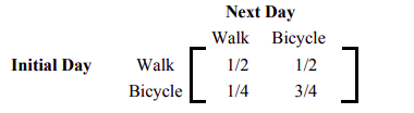
Professor Symons either walks to school, or he rides his bicycle. If he walks to school one day, then the next day, he will walk or cycle with equal probability. But if he bicycles one day, then the probability that he will walk the next day is 1/4. Express this information in a transition matrix.

Solution

We obtain the following transition matrix by properly placing the row and column entries. Note that if, for example, Professor Symons bicycles one day, then the probability that he will walk the next day is 1/4, and therefore, the probability that he will bicycle the next day is 3/4.

$Example10.1.3.png$

Example $\PageIndex{4}$

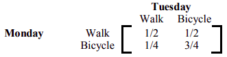
In Example $\PageIndex{3}$, if it is assumed that the initial day is Monday, write a matrix that gives probabilities of a transition from Monday to Wednesday.

Solution

If today is Monday, then Wednesday is two days from now, representing two transitions. We need to find the square, T², of the original transition matrix T, using matrix multiplication.

\[T=\left[\begin{array}{ll}
1 / 2 & 1 / 2 \\
1 / 4 & 3 / 4
\end{array}\right] \nonumber \]

\begin{aligned}
\mathrm{T}^{2}=\mathrm{T} \times \mathrm{T} &=\left[\begin{array}{lll}
1 / 2 & 1 / 2 \\
1 / 4 & 3 / 4
\end{array}\right] \left[ \begin{array}{l}
1 / 2 \\
1 / 4 & 1 / 2
\end{array}\right] \\
&=\left[\begin{array}{cc}
1 / 4+1 / 8 & 1 / 4+3 / 8 \\
1 / 8+3 / 16 & 1 / 8+9 / 16
\end{array}\right] \\
&=\left[\begin{array}{cc}
3 / 8 & 5 / 8 \\
5 / 16 & 11 / 16
\end{array}\right]
\end{aligned}

Recall that we do not obtain $T^2$ by squaring each entry in matrix $T$, but obtain $T^2$ by multiplying matrix $T$ by itself using matrix multiplication.

We represent the results in the following matrix.

$Example10.1.4.png$

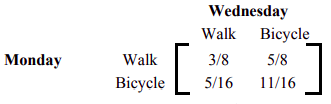
We interpret the probabilities from the matrix T² as follows:

P(Walked Wednesday | Walked Monday) = 3/8.
P(Bicycled Wednesday | Walked Monday) = 5/8.
P(Walked Wednesday | Bicycled Monday) = 5/16.
P(Bicycled Wednesday | Bicycled Monday) = 11/16.

Example $\PageIndex{5}$

The transition matrix for Example $\PageIndex{3}$ is given below.

$Example10.1.5.png$

Write the transition matrix from

Monday to Thursday
Monday to Friday.

Solution

a.) In writing a transition matrix from Monday to Thursday, we are moving from one state to another in three steps. That is, we need to compute T³.

\[\mathrm{T}^{3}=\left[\begin{array}{ll}
11 / 32 & 21 / 32 \\
21 / 64 & 43 / 64
\end{array}\right] \nonumber \]

b) To find the transition matrix from Monday to Friday, we are moving from one state to another in 4 steps. Therefore, we compute T⁴.

\[\mathrm{T}^{4}=\left[\begin{array}{ll}
43 / 128 & 85 / 128 \\
85 / 256 & 171 / 256
\end{array}\right] \nonumber \]

It is important that the student is able to interpret the above matrix correctly. For example, the entry 85/128, states that if Professor Symons walked to school on Monday, then there is 85/128 probability that he will bicycle to school on Friday.

There are certain Markov chains that tend to stabilize in the long run. We will examine these more deeply later in this chapter. The transition matrix we have used in the above example is just such a Markov chain. The next example deals with the long term trend or steady-state situation for that matrix.

Example $\PageIndex{6}$

Suppose Professor Symons continues to walk and bicycle according to the transition matrix given in Example $\PageIndex{3}$. In the long run, how often will he walk to school, and how often will he bicycle?

Solution

If we examine higher powers of the transition matrix T, we will find that it stabilizes.

\[\mathrm{T}^{5}=\left[\begin{array}{ll}
.333984 & 666015 \\
.333007 & .666992
\end{array}\right] \quad \mathrm{T}^{10}=\left[\begin{array}{ll}
.33333397 & .66666603 \\
.333333301 & .66666698
\end{array}\right] \nonumber \]

\[\text { And } \quad \mathrm{T}^{20}=\left[\begin{array}{ll}
1 / 3 & 2 / 3 \\
1 / 3 & 2 / 3
\end{array}\right] \quad \text { and } \mathrm{T}^{\mathrm{n}}=\left[\begin{array}{cc}
1 / 3 & 2 / 3 \\
1 / 3 & 2 / 3
\end{array}\right] \text { for } \mathrm{n}>20 \nonumber \]

The matrix shows that in the long run, Professor Symons will walk to school 1/3 of the time and bicycle 2/3 of the time.

When this happens, we say that the system is in steady-state or state of equilibrium. In this situation, all row vectors are equal. If the original matrix is an n by n matrix, we get n row vectors that are all the same. We call this vector a fixed probability vector or the equilibrium vector E. In the above problem, the fixed probability vector E is [1/3 2/3]. Furthermore, if the equilibrium vector E is multiplied by the original matrix T, the result is the equilibrium vector E. That is,

ET = E , or $\left[\begin{array}{lll}
1 / 3 & 2 / 3
\end{array}\right]\left[\begin{array}{cc}
1 / 2 & 1 / 2 \\
1 / 4 & 3 / 4
\end{array}\right]=\left[\begin{array}{ll}
1 / 3 & 2 / 3
\end{array}\right]$

Learning Objectives

Example \(\PageIndex{1}\)

Example \(\PageIndex{2}\)

Example \(\PageIndex{3}\)

Example \(\PageIndex{4}\)

Example \(\PageIndex{5}\)

Example \(\PageIndex{6}\)